© J. Debayle, published by EDP Sciences, 2019

1 Introduction

The mechanical and use properties of metal alloys depend on several factors, including the amount and the geometry of impurities (inclusions). In this context, image analysis enables these inclusions to be studied from digital images acquired by various systems such as electron microscopy or X-ray tomography.

This paper therefore aims to present some geometrical and morphometrical tools of image analysis, in order to characterize inclusions in metal alloys. To achieve this quantification, many geometrical and morphometrical features are traditionally used to quantitatively describe a population of objects (inclusions) [1,2].

Integral geometry [3–5], via Minkowski’s functionals [6] (in 2D: area, perimeter, Euler-Poincaré number), has been particularly investigated in image analysis. Indeed, integral geometry [3–5] has generalized convex geometry to finite unions of convex sets. This concept well applies to digital image analysis, since the smallest element (2D pixel) is indeed a convex set [7]. Nevertheless, they are sometimes insufficient for the characterization of complex microstructures (such as aggregates/agglomerates of objects) [8]. Other quantitative parameters are then necessary in order to discriminate or group different families of objects. In particular, shape diagrams [9–11] are mathematical representations in the Euclidean plane for studying the morphology (shape) of objects, regardless of their size. In addition, this representation also makes it possible to analyze the evolution from one shape to another. It also enables a convexity discrimination to be done with a direct visualization of the shape diagrams. For very complexe structures, such as fractal objects, other descriptors could be required. Indeed, these geometrical and morphometrical descriptors could be insufficient (as it stands) to analyse such strutures but the proposed measurements can be computed on some geometrical transformations of the object to be studied, providing some measurements functions and not only scalars. This kind of approach has been particularly studied in [12]. Other descriptors are based on computational geometry and stochastic geometry [13] but they will not be studied in this paper.

The following of the paper is organized as follows: Section 2 gives the fundamentals notions of the Minkowski functionals. The computational aspects as well as the properties and the limitations of these functionals are done. Section 3 presents the shape diagrams and some illustration of the properties of continuity and convexity discrimination are done. The last section concludes this work. The objective of this paper is not to give an exhaustive list of geometrical and morphometrical tools, but rather to focus on specific descriptors with a compact representation and good mathematical properties and which are easy to compute.

2 Geometrical tools via integral geometry

Convex geometry, based on Minkowski functionals [6], allows to geometrically characterize a convex set in ${\mathrm{ℝ}}^{\mathit{n}}$. There are exactly n + 1 Minkowski functionals, satisfyinging certain properties (additivity, continuity, invariance by displacements). For example on ${\mathrm{ℝ}}^2$, these functionals are the area, the perimeter and the Euler number. The two first functionals are related to well-known geometrical characteristics while the Euler number is a topological characteristic corresponding to the number of connected components minus the number of holes inside the set. The Minkowski functionals provide a basis of measurements in ${\mathrm{ℝ}}^{\mathit{n}}$ [14]. They are therefore linearly independent and any other functional satisfying these properties is a linear combination of these properties. Integral geometry [3–5] has generalized convex geometry to finite unions of convex sets. This concept well applies to digital image analysis, since the smallest element (2D pixel) is indeed a convex set [7]. In the following, an efficient method (based on discrete geometry) for computing these Minkowski functionals from a 2D binary image is given [12]. Thereafter, the properties of the Minkowski functionals and their limitations will be presented.

2.1 Notions of discrete geometry

2.1.1 Digital topology

Let X be a two-dimensional binary image of  size ${\mathit{l}}_1\times {\mathit{l}}_2,({\mathit{l}}_1,{\mathit{l}}_2)\in {\mathrm{\mathbb{N}}}^2$. The spatial support of X is denoted $\mathrm{D}=[0,{\mathit{l}}_1]\cap \mathrm{\mathbb{N}}\times [0,{\mathit{l}}_2]\cap \mathrm{\mathbb{N}}$. X is represented by a matrix $\mathit{B}={({\mathit{b}}_{\mathit{x}})}_{\mathit{x}\in \mathit{D}}$, where b_x, belonging to {0,1}, is the value of the intensity of the pixel (abbreviated as “picture element”, the most small image element) of coordinates x ∈ D. By convention, the object and background of the image are represented by pixels of intensity b_x = 1 and b_x = 0, respectively. In particular, a set of connected pixels included in the object is a hole. The notion of neighbourhood induces topology on D:

• two pixels of the object (or background) with coordinates ${\mathit{x}}^1=({\mathit{x}}_1^1,{\mathit{x}}_2^1)$  and ${\mathrm{x}}^2=({\mathrm{x}}_1^2,{\mathrm{x}}_2^2)$ are 4-adjacent if and only if $|{\mathrm{x}}_1^1-{\mathrm{x}}_1^2|+|{\mathrm{x}}_2^1-{\mathrm{x}}_2^2|=1$;

• two pixels of the object (or background) with coordinates ${\mathit{x}}^1=({\mathit{x}}_1^1,{\mathit{x}}_2^1)$ and ${\mathrm{x}}^2=({\mathrm{x}}_1^2,{\mathrm{x}}_2^2)$ are 8-adjacents if and only if max $(|{\mathrm{x}}_1^1-{\mathrm{x}}_1^2|,|{\mathrm{x}}_2^1-{\mathrm{x}}_2^2|)=1$.

The p-neighbourhood (p = 4 or p = 8) of a pixel is therefore defined as the set of pixels p-adjacent to this one [Ros74]. The notion of neighbourhood makes it possible to establish the notion of connectedness [15]. Indeed, two pixels of the object (or background) are p-connected (p = 4 or p = 8) if there is a path of p-adjacent pixels connecting them. Similarly, a related component in a two-dimensional binary image is a set of adjacent pixels forming a path in the image. In order to satisfy Jordan’s theorem, the connections must be different for the background pixels and for the object pixels. Therefore, these two-dimensional image connections are noted (4, 8) or (8, 4), the first coordinate corresponding to the object, and the second one at the bottom [16].

2.1.2 Cell configuration

The “physical” spatial support of the image (i.e. the “continuous” spatial support) is covered by cells associated with pixels. A cell (size square the interpixel distance) is composed of one face, four edges and four vertices. Either a cell is centered in a pixel (cell intrapixel), or a cell is built by connecting pixels (interpixel cell). Figure 1 illustrates the overlapping of an image consisting of sixteen pixels, and its two possible representations.

4- and 8-adjacence are associated with the cell representation:

• using intrapixel cells, two pixels of the object (background) are adjacent if and only if their respective cells have a common vertex (8-adjacence);

• using interpixel cells, two pixels of the object (background) are adjacent if and only if they share the same edge (4-adjacence).

Figure 2 shows the two cell representations of the two-dimensional binary image X associated with matrix B.

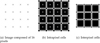Fig. 1 Image composed of sixteen pixels (a) represented by crosses (×). The image is covered by intrapixel (b) or interpixel (c) cells, composed of vertices, edges and faces (vertice = ●, edge = –, face = ■). Note: image (a) is covered by sixteen intrapixel cells or nine interpixel cells [12].

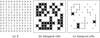Fig. 2 Representation of intrapixel (b) and interpixel (c) cells of the binary image X associated to the matrix B (a) [12].

2.1.3 Neighborhood configuration

In order to efficiently calculate the number of vertices v, edges e and faces f of the object (pixels of intensities equal to 1), the different neighbourhood configurations (size two by two pixels) of the original image X are determined [1,2,17–22]. Thus, to each pixel corresponds a neighborhood. In addition, sixteen configurations are possible (Tab. 1 where the values 0 and 1 represent the intensity of the pixels (1: object, 0: background).

Then, each configuration contributes for a known number of vertices, edges and faces (Eqs. (1–3)). To determine the neighborhood configurations of all pixels, an efficient algorithm consists in convolving the binary matrix B (associated with the image X) by a mask F of dimension two, whose values are powers of two, and whose origin is the pixel at the top left with value 1:

 $F\mathrm{}=\left(\begin{array}{cc}\hfill 1\hfill & \hfill 4\hfill \\ \hfill 2\hfill & \hfill 8\hfill \end{array}\right)$

Each value $\alpha \in [0,15]\cap \mathrm{\mathbb{N}}$ of the resulting matrix B * F, where * denotes the convolution operator, corresponds to a known neighborhood configuration. Table 1 shows the possible configurations (1: object, 0: background) and the associated values α resulting from the convolution. The histogram h of B*F gives the distribution of the neighborhood configurations of the X image. And each configuration contributes to a known number of vertices, edges and faces: $$v\mathrm{}{\displaystyle =\sum _{\alpha =0}^{15}}{v}_{\alpha }h\mathrm{}(\alpha \mathrm{})\text{,}$$(1) $$\mathit{e}\mathrm{}{\displaystyle =\sum _{\alpha =0}^{15}}{\mathit{e}}_{\alpha }h\mathrm{}(\alpha \mathrm{})\text{,}$$(2) $$f=\mathrm{}{\displaystyle \sum _{\alpha =0}^{15}}{f}_{\alpha }h\mathrm{}(\alpha )\mathrm{}\text{,}$$(3) where for $\alpha \in [0,15]\cap \mathrm{\mathbb{N}}$, v_α, e_α and f_α are the coefficients of the linear combinations, depending on the image overlap, given in Table 2.

2.2 Minkowski functionals

Based on these notions of discrete geometry, the different Minkowski functionals can be computed from the number of vertices v, edges e and faces f.

2.2.1 Euler number

The Euler number, denoted χ, corresponding to the number of connected components minus the number of holes, can be computed from the image overlap by cells: $$\chi \mathrm{}=v-e+f\text{,}$$(4) where v , e and f are the number of vertices, edges and faces, respectively.

It is important to note that equation (4) gives different numbers of Eulerχ, depending on the representation of cells. The representation of intrapixel (or interpixel) cells gives the result with (8, 4)-connexity (respectively (4, 8)-connexity). Each configuration of neighbourhoods contributes to a known number of vertices, edges and faces, and therefore for the number of Euler. Thanks to equations (1–4), the number of Euler is calculated as follows: $${\chi }^{(8,4)}\mathrm{}{\displaystyle =\sum _{\alpha =0}^{15}}{\chi }_{\alpha }^{(8,4)}h\mathrm{}(\alpha \mathrm{}\text{),}$$(5) $${\chi }^{(4,8)}\mathrm{}{\displaystyle =\sum _{\alpha =0}^{15}}{\chi }_{\alpha }^{(4,8)}h\mathrm{}(\alpha \mathrm{}\text{),}$$(6) where χ_α = v_α − e_α + f_α is given in the Table 2. The Euler number is then efficiently computed by using the coefficients associated to each configuration, depending on the image overlap.

2.2.2 Perimeter

Two methods, giving different results, allow to estimate the perimeter of an object. Using intrapixel cells, the perimeter, denoted P is determined by counting the number of edges common to two pixels of different intensities, thanks to the following formula: $$P\mathrm{}=-4f+2e\text{.}$$(7)

The discretization implies that this perimeter is underestimated. Following the equations (1–3), P is computed as: $$P=\mathrm{}{\displaystyle \sum _{\alpha =0}^{15}}{P}_{\alpha }h\mathrm{}(\alpha )\mathrm{}\text{,}$$(8) where P_α = v_α − e_α + f_α is given in the Table 2.

The Crofton perimeter, denoted ${\displaystyle \bar{P}}$ independent of the representation of the cells used, gives a better estimation. It associates the length of a curve with the number of times a “random” line intersects the set [23]. Let γ be a planar curve, l a line oriented in direction φ and of length p, n_γ (l) the number of points at which γ and l intersect. Crofton’s formula expresses the arc length of the γ curve in terms of the spatial integral of all oriented lines: $$\text{length(}\mathrm{}\gamma )=\mathrm{}\frac{1}{4}\int \int n_{\gamma }\mathrm{}(\varphi \mathrm{},p)\mathrm{}d\varphi dp,$$

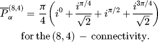
In the discrete case, only the angle orientations 0, $\frac{\pi }{4}$, $\frac{\pi }{2}$, and $\frac{3\pi }{4}$ are considered; they are chosen according to the connectivity. The number of intercepts for each of these lines is counted, and denoted respectively i⁰, i^π/4, i^π/2 and i^3π/4. They are then standardized by 1 or $\sqrt{2}$ depending on the orientation. The average is finally calculated by multiplying by π, a value representing the integral of the orientations, and by dividing by the number of orientations used. The Crofton perimeter is then calculated as follows: $${{\displaystyle \overline{P}}}_{\alpha }^{(4,8)}\mathrm{}=\frac{\pi }{2}\left(i^0+i^{\pi /2}\right)\mathrm{f}\mathrm{o}\mathrm{r}\mathrm{t}\mathrm{h}\mathrm{e}\mathrm{(}\mathrm{4,8}\mathrm{)}-\mathrm{c}\mathrm{o}\mathrm{n}\mathrm{n}\mathrm{e}\mathrm{c}\mathrm{t}\mathrm{i}\mathrm{v}\mathrm{i}\mathrm{t}\mathrm{y}\text{,}$$(9) $${{\displaystyle \overline{P}}}_{\alpha }^{(8,4)}=\mathrm{}\frac{\pi }{4}\left(i^0+\frac{i^{\pi /4}}{\sqrt{2}}+i^{\pi /2}+\frac{i^{3\pi /4}}{\sqrt{2}}\right)\mathrm{f}\mathrm{o}\mathrm{r}\mathrm{t}\mathrm{h}\mathrm{e}\mathrm{(}\mathrm{8,4}\mathrm{)}-\mathrm{c}\mathrm{o}\mathrm{n}\mathrm{n}\mathrm{e}\mathrm{c}\mathrm{t}\mathrm{i}\mathrm{v}\mathrm{i}\mathrm{t}\mathrm{y}\text{.}$$(10)

This perimeter is computed thanks to the following linear combinations that provide coefficients to the different numbers of intercepts. $${{\displaystyle \overline{P}}}_{\alpha }^{(4,8)}\mathrm{}{\displaystyle =\sum _{\alpha =0}^{15}}{{\displaystyle \overline{P}}}_{\alpha }^{(4,8)}h\mathrm{}(\alpha )\mathrm{}\text{,}$$(11) $${{\displaystyle \overline{P}}}_{\alpha }^{(8,4)}\mathrm{}{\displaystyle =\sum _{\alpha =0}^{15}}{{\displaystyle \overline{P}}}_{\alpha }^{(8,4)}h\mathrm{}(\alpha )\mathrm{}\text{,}$$(12) where the coefficients ${{\displaystyle \overline{P}}}_{\alpha }^{(4,8)}\mathrm{}$ and ${{\displaystyle \overline{P}}}_{\alpha }^{(8,4)}\mathrm{}$ are given in Table 2.

For wired objects, considered as objects of dimension one, the two previously defined perimeters do not give robust results, since they double the length of a line.

2.2.3 Area

The area (or surface), denoted A, of the set is generally defined by the number of pixels of the set. According to the representation of the cells, it is then equal to the number of vertices v (interpixel cells) or the number of faces f (intrapixel cells), the result being always the same. Generally, this overestimates the area. Thanks to equations (1–3), the area A is calculated as follows: $$A\mathrm{}{\displaystyle =\sum _{\alpha =0}^{15}}{A}_{\alpha }h\mathrm{}(\alpha \mathrm{})\text{,}$$(13) where the coeffcients A_α are given in Table 2.

It is also possible to count the number of faces f obtained with the representation of the interpixel cells. In this case, the area is generally underestimated, but the wired objects have no area (they are therefore considered as objects of dimension one), this result being more robust.

2.3 Properties

The n + 1 Minkowski functionals MF satisfy the following properties, for all compact convex sets X and Y in ${\mathrm{ℝ}}^{\mathit{n}}$:

• increasingness: X ⊆ Y ⇒ MF (X) ≤ MF (Y);

• invariance to rigid transformations t: MF (X) = MF (X_t) where X_t denotes the transformation of X by the rigid operator t (translation and rotation);

• homogeneity: MF (λX) = λ^dMF (X) for $\lambda \in \mathrm{ℝ}$ and d the dimensionnality of MF;

• additivity: MF (X) + MF (Y) = MF (X ∪ Y) + MF (X ∩ Y);

• continuity: ${{\displaystyle lim}}_{i\to +\infty }{d}_H\mathrm{}(X_i\mathrm{},X)=0\Rightarrow {{\displaystyle lim}}_{i\to +\infty }MF\mathrm{}(X_i\mathrm{})MF\mathrm{}(X)\mathrm{}$ where d_H denotes the Hausdorff distance [DD06] and ${\mathrm{}(X_i)\mathrm{}}_i$ denotes a family of convex sets.

Among these five properties, three are still valid for the finite unions of convex sets: invariance by rigid transformation, homogeneity and additivity.

Regarding Hadwiger’s theorem [14], one other main important property is that any homogeneous and continuous functional that is invariant under rigid motions can be represented as a sum of the n + 1 Minkowski functionals. In ${\mathrm{ℝ}}^2$, it means that such a functional μ computed on a set X can be expressed as: $$\mu \mathrm{}(X\mathrm{})=c_0\chi \mathrm{}(X\mathrm{})+c_{1}P\mathrm{}(X)\mathrm{}+c_{2}A\mathrm{}(X\mathrm{})\text{,}$$(14) where c₀ , c₁ and c₂ are real-valued coefficients.

2.4 Limitations

Integral geometry provide useful and efficient tools for the geometrical characterization of sets via the Minkowski functionals. Neverthess, they are not enough to discriminate complex spatial structures [8], as shown in Figure 3.

It is then necessary to provide other characteristics to be able to discriminate these spatial structures. In the literature, there exists a lot of other characteristics. In the following, morphometrical functionals, and more particularly shape diagrams, will be presented. The advantage is that they have a compact representation, some good mathematical properties and a low computational cost.

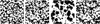Fig. 3 Four binary images (300 × 300 pixels or 1 × 1 mm) of borosilicate glass visually different but having the same Minkowski functionals [8]: area 0.437 mm2, perimeter 30.28 mm, number of Euler 11 or 16 depending on the connectivity).

3 Morphometrical tools via shape diagrams

Shape diagrams [9–11] are representations in the Euclidean plane introduced to study the morphology of 2D connected compact sets. Such a set is represented by a point within a shape diagram whose coordinate axes are morphometrical functionals defined as normalized ratios of geometrical functionals. In this section, the construction of the shape diagrams will be firstly given. The second part will be focused on some properties of continuity and convexity discrimination.

3.1 Morphometrical functionals

In addition to area A and perimeter P, other geometrical functionals have been studied such as the radii r and R of the inscribed and circumscribed circles respectively, and the minimum and maximum Feret diameters and d respectively [24]. The Feret diameter is a measure of an object size along a specified direction. In general, it can be defined as the distance between the two parallel planes restricting the object perpendicular to that direction. It is therefore also called the caliper diameter, referring to the measurement of the object size with a caliper. ω and d are the minimal and maximal diameter on the different possible orientations. Figure 4 illustrates these four additional geometrical functionals.

In practice, the Feret diameters are easily determined by firstly computing the convex hull of the object. Indeed, the Feret diameters for an object and for its convex hull are equal. The convex hull being a polygon, one can use the “rotating callipers” algorithm [25] to directly determine the largest and smallest projections.

For a connected compact set, the relationships between these geometrical functionals are constrained by geometric inequalities [26,27]. These geometric inequalities link geometrical functionals by pairs. Futhermore, they allow to determinate the morphometrical functionals (Tab. 3).

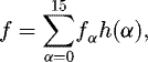
The morphometrical functionals are invariant under similitude transformations (consequently, they do not depend on the global size of the set) and are defined as ratios between two geometrical functionals. In these ratios, the units of the numerator and the denominator are dimensionally homogeneous and the result has therefore no unit. Moreover, a normalization by a constant value (scalar multiplication) allows to have a ratio that ranges within [0,1]. For each morphometrical functional, the scalar value depends directly on the associated geometric inequality [28]. In total, there are fifteen morphometrical functionals for a connected compact set.   $4\mathrm{\pi }\mathit{A}/{\mathit{P}}^2$, r/R, ω/d and 4R/P are four examples of these morphometrical functionals. Their concrete meanings are the roundness, the circularity, the diameter constancy and the thinness, respectively.

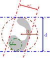Fig. 4 Geometrical functionals: radii of inscribed (r) and circumscribed (R) circles, minimum (ω) and maximum (d) Feret diameters.

3.2 Shape diagrams

Shape diagrams can be defined by these fifteen morphometrical functionals. Each shape diagram enable to represent the morphometry of any connected compact set from two morphometrical functionals (that is to say from three geometrical functionals because the two denominators use the same geometrical functionals).

Let be any triplet of the considered six geometrical functionals (A, P, r, R,ω, d) and (M₁, M₂) be some particular morphometrical functionals valued in [0.1]². A shape diagram  $D$ is represented in the plane domain [0.1]² (whose axis coordinates are the morphometrical functionals M₁ and M₂) where any connected compact set $S$  is mapped onto a point (x, y). Mathematically, a shape diagram $D$ is obtained from the following mapping: 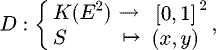$$D:\{\begin{array}{c}K(E^2)\\ S\end{array}\begin{array}{c}\to \\ \mapsto \end{array}\begin{array}{c}{\begin{array}{c}[0,1]\end{array}}^2\\ (\mathit{x},\mathit{y})\end{array},$$ where $\mathrm{}{K(E}^2)\mathrm{}$ denotes the compact sets of the Euclidean 2D plane. Using all the fifteen morphometrical functionals, twenty-two shape diagrams are defined, denoted 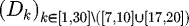${\left(D_{\mathit{k}}\right)}_{k\in [1,30]\backslash (\mathrm{}[7,10]\cup [17,20])\mathrm{}}$, respectively (Tab. 4).

Some geometric inequalities, and consequently some shape diagrams, are restricted to convex shapes [29], that are not considered in this paper. A detailed comparative study has been performed in order to analyze the representation relevance of these twenty-two shape diagrams [29–31].

For example, the shape diagram 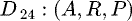$D{\hspace{0.17em}}_{24}\mathrm{}:(A\mathrm{},R\mathrm{},P\mathrm{})$ is obtained from the following mapping. $$D_{24}(\mathrm{A},\mathrm{R},\mathrm{P}):\{\begin{array}{c}K({\mathrm{E}}^2)\\ S\end{array}\begin{array}{c}\to \\ \mapsto \end{array}\begin{array}{c}{\begin{array}{c}[0,1]\end{array}}^2\\ (\frac{4\mathrm{\pi }\mathrm{A}}{{\mathrm{P}}^2},\frac{4\mathrm{R}}{\mathrm{P}})\end{array},$$

The concrete meanings of the morphometrical functionals 4πA/P² and 4R/P are the roundness and the thinness, respectively.

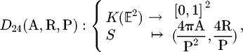
Figure 5 illustrates three shape diagrams where some elementary sets are mapped.

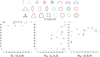Fig. 5 Illustration of three specific shape diagrams where 24 elementary sets are mapped. It shows that some diagrams (using some specific morphometrical functionals) are not suitable for shape discrimination and classification. For example, different shapes can be located on the same place within the diagram $D_{12}$, highlighting the non-unicity of such a representation.

3.3 Properties

The properties of the different shape diagrams have been studied in [29–31]. In the following, the properties of continuity and convexity discrimination are presented in order to show the better relevance of some shape diagrams.

3.3.1 Continuity

Let two 2D connected compact sets and the connected compact set class allowing to switch from one to the other using a degree of freedom of the set. For example, the semi-circle goes to the semi-disk through semi-rings whose the cavity radius decreases (Fig. 6).

For each pair i of sets, a class C_i of connected compact sets with one degree of freedom could be defined. Thus, a curve denoted $C_{\mathit{i},\mathit{k}}$ from each simply connected compact set class C_i is created in each shape diagram $D_{\mathit{k}}$. These curves are related to the continuity of the shape diagram with respect to a small deformation of the set. This process can be used for elementary some pairs of connected compact sets.

In the following Figure 7, eight classes of connected compact sets are illustrated on three shape diagrams. It shows the location of the continuity curves from one shape to another.

A detailed study of this property can be found in [29–31].

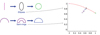Fig. 6 Illustration of the sets (represented by a curve on the shape diagrams) coming from a transformation (using a degree of freedom of the set) from one set to another [12].

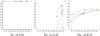Fig. 7 Illustration of eight continuity curves (representing the locations of the transformed sets from one set to another) onto three shape diagrams [12].

3.3.2 Convexity discrimination

The convexity discrimination first requires the definition of the shape convexity. A set is convex when the line segment which joins any two points in it lies totally within the set. In other terms, the shape convexity could be quantified with the probability that two points in the set lies totally within it. Convexity parameters are commonly used in the analysis of shapes. The measurement value of the shape convexity of any set ranges between 0 and 1 (it is a probability). A convex set gives the value 1. Futhermore, the less the parameter value is high, the less the shape is convex. The convexity measurement can be computed, for instance, by the ratio c = A/A_c where A_c is the area of the convex hull of the set. This convexity parameter c has the following desirable properties:

• its value is always a number within [0,1]:

• its value is 1 if and only if the set is convex;

• it is invariant under similitude transformations;

• there is a simple and fast computing algorithm.

Figure 8 shows this convexity parameter for some specific sets. The colormap corresponds to the different values of this parameter from 0 (black) to 1 (dark red), i.e from non-convex sets to convex sets.

Figure 9 illustrates three shape diagram where 1370 various discrete sets are mapped, and on which the boundaries of the convex domain are superimposed (the domain where all compact convex sets are located [11,28]).

One can see that the shape diagram $D_{24}$ presents a good convexity discrimination [31]. The sets mapped at the bottom left (sets with both low roundness values and low thinness values) are strongly concave, whereas the sets mapped at the top (sets with high thinness values) are stongly convex. In the two other shape diagrams, it would be more difficult to discriminate the convexity of the sets since the different color points are much more mixed.

A more detailed study, including other properties of the shape diagrams, can be found in [29–31]. Among the different shape diagrams, it has been shown that the shape diagram $D{\hspace{0.17em}}_{24}\mathrm{}:(A\mathrm{},R\mathrm{},P)\mathrm{}$ is a good candidate for shape analysis regarding its representation relevance and discrimination power.

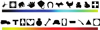Fig. 8 Illustration of the convexity parameter for some specific sets. The colormap corresponds to the different values of this parameter from 0 (black) to 1 (dark red), i.e from non-convex sets to convex sets [12].

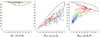Fig. 9 Family of 1370 discrete sets which are mapped onto three shape diagrams. The colormap corresponds to the different values of the convexity parameter from 0 (black) to 1 (dark red) of the sets, i.e from non-convex sets to convex sets [12].

4 Conclusions

The purpose of this paper was to propose geometrical and morphometrical tools for characterizing inclusions in metal alloys from digital images acquired by various systems such as electron microscopy or X-ray tomography. The objective was not to give an exhaustive list of geometrical and morphometrical tools, but rather to focus on specific descriptors. In this context, the Minkowski functionals (geometrical tools) and the shape diagrams (morphometrical tools) have been presented. It has been shown that these descriptors have a compact representation, are computationnaly effective and have some good mathematical properties. For sure, they could be insufficient (as it stands) to analyse very complex strutures but the proposed measurements can be computed on some geometrical transformations of the object to be studied, providing some measurements functions and not only scalars. This kind of approach has been particularly studied in [12]. In conclusion, image analysis using integral geometry and shape diagrams provide efficient tools to quantitatively describe inclusions (providing separate information on size and shape). The geometrical characteristics of these inclusions could thereafter be related to the mechanical properties of the metal alloys.

References

All Tables

All Figures

	Fig. 1 Image composed of sixteen pixels (a) represented by crosses (×). The image is covered by intrapixel (b) or interpixel (c) cells, composed of vertices, edges and faces (vertice = ●, edge = –, face = ■). Note: image (a) is covered by sixteen intrapixel cells or nine interpixel cells [12].
In the text

	Fig. 2 Representation of intrapixel (b) and interpixel (c) cells of the binary image X associated to the matrix B (a) [12].
In the text

	Fig. 3 Four binary images (300 × 300 pixels or 1 × 1 mm) of borosilicate glass visually different but having the same Minkowski functionals [8]: area 0.437 mm2, perimeter 30.28 mm, number of Euler 11 or 16 depending on the connectivity).
In the text

	Fig. 4 Geometrical functionals: radii of inscribed (r) and circumscribed (R) circles, minimum (ω) and maximum (d) Feret diameters.
In the text

	Fig. 5 Illustration of three specific shape diagrams where 24 elementary sets are mapped. It shows that some diagrams (using some specific morphometrical functionals) are not suitable for shape discrimination and classification. For example, different shapes can be located on the same place within the diagram $D_{12}$, highlighting the non-unicity of such a representation.
In the text

	Fig. 6 Illustration of the sets (represented by a curve on the shape diagrams) coming from a transformation (using a degree of freedom of the set) from one set to another [12].
In the text

	Fig. 7 Illustration of eight continuity curves (representing the locations of the transformed sets from one set to another) onto three shape diagrams [12].
In the text

	Fig. 8 Illustration of the convexity parameter for some specific sets. The colormap corresponds to the different values of this parameter from 0 (black) to 1 (dark red), i.e from non-convex sets to convex sets [12].
In the text

	Fig. 9 Family of 1370 discrete sets which are mapped onto three shape diagrams. The colormap corresponds to the different values of the convexity parameter from 0 (black) to 1 (dark red) of the sets, i.e from non-convex sets to convex sets [12].
In the text

References

- J. Ohser, F. Mücklich, Statistical analysis of microstructures in materials science, John Wiley and Sons, New York, USA, 2000 [Google Scholar]
- J. Ohser, K. Schladitz, Image processing and analysis, Clarendon Press Oxford, Oxford, UK, 2006 [Google Scholar]
- W. Blaschke, Vorlesungen über integralgeometrie, VEB, Berlin, 1955 [Google Scholar]
- K.R. Mecke, Integral geometry in statistical physics, Int. J. Mod. Phys. B 12(9), 861–899 (1998) [Google Scholar]
- L.A. Santalo, Integral geometry and geometric probability, Cambridge University Press, Cambridge, UK, 2004 [CrossRef] [Google Scholar]
- H. Minkowski, Volumen und oberfläche, Math. Ann. 57, 447–495 (2003) [Google Scholar]
- K.R. Michielsen, H. De Raedt, Integral-geometry morphological image analysis, Phys. Rep. 347, 461–538 (2001) [Google Scholar]
- V. Schulz, Description and reconstruction of microscopic random heterogenous media in order to estimate macroscopic hydraulic functions, PhD thesis, University of Heidelberg, 2003 [Google Scholar]
- W. Blaschke, Konvexe Bereiche gegebener konstanter Breite und kleinsten Inhalts, Math. Ann. 76, 504–513 (1915) [Google Scholar]
- W. Blaschke, Eine frage über konvexe körper, Jahresbericht Deutsch, Math.-Verein. 25, 121–125 (1916) [Google Scholar]
- L.A. Santalo, Sobre los sistemas completos de desigualdades entre tres elementos de una figura plana, Math. Notae. 17, 82–104 (1961) [Google Scholar]
- S. Rivollier, Analyse d’image géométrique et morphométrique par diagrammes de forme et voisinages adaptatifs généraux, PhD thesis, École Nationale Supérieure des Mines de Saint-Étienne, France, 2010 [Google Scholar]
- S.N. Chiu, D. Stoyan, W. Kendall, J. Mecke, Stochastic geometry and its applications, John Wiley & Sons, Chichester, UK, 2013 [Google Scholar]
- H. Hadwiger, Vorlesungen über inhalt, oberfläsche und isoperimetrie, Springer-Verlag, Berlin Heidelberg, Germany, 1957 [CrossRef] [Google Scholar]
- A. Rosenfeld, Connectivity in digital pictures, J. ACM 17(1), 146–160 (1970) [CrossRef] [Google Scholar]
- A. Rosenfeld, A converse to the jordan curve theorem for digital curves, Inf. Control 29, 292–293 (1975) [CrossRef] [Google Scholar]
- W. Nagel, J. Ohser, K. Pischang, An integral-geometric approach for the euler-poincaré characteristic of spatial images, J. Microsc. 198, 54–62 (2000) [CrossRef] [PubMed] [Google Scholar]
- C. Lang, J. Ohser, R. Hilfer, On the analysis of spatial binary images, J. Microsc. 203(3), 303–313 (2001) [CrossRef] [PubMed] [Google Scholar]
- J. Ohser, W. Nagel, K. Schladitz, The Euler number of discretised sets – On the choice of adjacency in homogeneous lattices, in: Morphology of condensed matter, Springer-Verlag, Berlin Heidelberg, Germany, 2002, pp. 275–798 [CrossRef] [Google Scholar]
- J. Ohser, W. Nagel, K. Schladitz, The euler number of discretised sets– Surprising results in three dimensions, Imag. Anal. Stereol. 22, 11–19 (2003) [CrossRef] [Google Scholar]
- K. Schladitz, J. Ohser, W. Nagel, Measuring intrinsic volumes in digital 3d images, Discret. Geom. Comp. Imag. 4245, 247–258 (2006) [CrossRef] [Google Scholar]
- K. Sandfort, J. Ohser, Labeling of n-dimensional images with choosable adjacency of the pixels, Imag. Anal. Stereol. 28, 45–61 (2009) [Google Scholar]
- M.W. Crofton, On the theory of local probability, applied to straight lines drawn at random in a plane, Philos. Trans. R. Soc. Lond. 158, 181–199 (1868) [Google Scholar]
- L.R. Feret, La grosseur des grains des matières pulvérulentes, Premières Communications de la Nouvelle Association Internationale pour l’Essai des Matériaux, Groupe D, 1930, pp. 428–436 [Google Scholar]
- M.I. Shamos, Computational geometry, PhD thesis, Yale University, 1978 [Google Scholar]
- Y.D. Burago, V.A. Zalgaller, Geometric inequalities, Springer-Verlag, Berlin Heidelberg, Germany, 1988 [CrossRef] [Google Scholar]
- P.R. Scott, P.W. Awyong, Inequalities for convex sets, Inequal. Pure Appl. Math. 1(1–6), 1–6 (2000) [Google Scholar]
- M.A.H. Cifre, G. Salinas, S.S. Gomis, Complete systems of inequalities, Inequal. Pure Appl. Math. 2(1), 1–12 (2001) [Google Scholar]
- S. Rivollier, J. Debayle, J.C. Pinoli, Shape diagrams for 2D compact sets – Part I: analytic convex sets, Aust. J. Math. Anal. Appl. 7(2–3), 1–27 (2010) [Google Scholar]
- S. Rivollier, J. Debayle, J.C. Pinoli, Shape diagrams for 2D compact sets – Part II: analytic simply connected sets, Aust. J. Math. Anal. Appl. 7(2–4), 1–21 (2010) [Google Scholar]
- S. Rivollier, J. Debayle, J.C. Pinoli, Shape diagrams for 2D compact sets – Part III: convexity discrimination for analytic and discretized simply connected sets, Aust. J. Math. Anal. Appl. 7(2–5), 1–18 (2010) [Google Scholar]
Cite this article as: Johan Debayle, Geometrical and morphometrical tools for the inclusion analysis of metallic alloys, Metall. Res. Technol. 116, 508 (2019)
All Tables
The twenty two shape diagrams axes coordinates for 2D simply connected compact sets.