| Issue |
Metall. Res. Technol.
Volume 114, Number 6, 2017
|
|
|---|---|---|
| Article Number | 607 | |
| Number of page(s) | 9 | |
| DOI | https://doi.org/10.1051/metal/2016065 | |
| Published online | 19 September 2017 | |
Regular Article
Methodology to assess fracture during crash simulation: fracture strain criteria and their calibration
1
ArcelorMittal Maizières Research SA, Voie Romaine,
BP30320,
57283
Maizières-les-Metz, France
2
ArcelorMittal, Automotive Products Development,
17 avenue des tilleuls,
57190
Florange, France
* e-mail: This email address is being protected from spambots. You need JavaScript enabled to view it.
Received:
10
June
2016
Received in final form:
4
November
2016
Accepted:
9
November
2016
Abstract
The use of Advanced High Strength Steels (AHSS) has greatly increased this last decade in the automotive industry. Because of their crash performance and their weight saving potential, these grades constitute a possible solution to achieve the safety and environmental regulations objectives. Nevertheless, the increase of tensile strength of these materials is generally associated with a loss of ductility compared to conventional steels. Thus, the prediction of their failure in crash loading conditions become of great importance for the design of vehicles. This paper proposes to calibrate for any AHSS, as Dual-Phase or Press Hardened Steels, different failure criteria, available in finite element software. First, specific tests and methodologies for strain measurement needed for models calibration are exposed. Second, an overview of these tested models and the procedure applied to take into account mesh dependency are provided. Finally, simulations results are compared with experiment on a real automotive component.
Key words: failure characterization / failure prediction / crash / LS-DYNA / CrachFEM
© EDP Sciences, 2017
1 Introduction
In order to achieve the safety and environmental regulations objectives, the Advanced High Strength Steels (AHSS) considerably and continuously increases in the automotive industry due to their crash performance and their weight saving potential. Nevertheless, the increase of tensile strength of these materials is generally associated with a loss of ductility compared to conventional steels, and the assessment of their failure in crash loading conditions becomes of prime importance for the steel supplier ArcelorMittal in order to their customers achieve a safe crash design of their vehicles [1].
For this purpose, numerous failure criteria are implemented in the finite element code LS-DYNA [2]. They are defined within MAT224 [2], MAT123 [2] or CrachFem [3] crash failure model cards. They can be formulated in different manners, according to strains or stresses, but it remains possible to compare them in plane stress conditions using the curve representation of the fracture strain according to stress triaxiality [4]. The accuracy of the failure prediction depends therefore mainly on this curve, and its reliable determination, at least for the range of stress states corresponding to the investigated loading.
The determination of this curve for different AHSS, as Dual Phase or Press Hardened Steels is proposed in this paper. The accuracy of failure prediction is then assessed by comparison between simulations and experiments on a real automotive component.
2 Fracture strain measurement
In this part, experimental determination of fracture strain regarding three loading paths is detailed:
-
the uniaxial tensile test,
-
an equibiaxial expansion test,
-
a plane strain test.
2.1 The uniaxial tensile test
2.1.1 Tensile specimen with hole
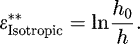
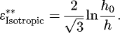
The uniaxial specimen used at ArcelorMittal is widely inspired from the specimen used by MatFEM [3]. It is designed with a hole as shown in Figure 1. The hole should prevent the specimen from necking and facilitate a ductile normal failure under uniaxial tensile conditions. The fracture strain can be measured by thickness reduction by looking at the broken cross section as illustrated in Figure 2(a) or by Digital Image Correlation in Figure 2(b) (DIC using ARAMIS system [5]). Assuming isotropic plasticity, the local failure strain is directly derived from final and initial thickness ratio, i.e. as defined in equation (1) where h0 is the initial thickness, and h is the reduced thickness at the failure position:
 (1)
(1)
This result is not strictly true since the strain path is not direct until the failure occurs and the triaxiality generally increases just before the fracture.
The advantage of this method is its relative simplicity. Unfortunately, the impact of the measurement precision is very important: 10% of uncertainty on the final thickness leads to more than 20% of uncertainty on the failure strain, which remains very high.
It has been demonstrated that, because of very high strain gradients, measurement with micrometer is not accurate enough. It is very difficult to capture the thickness right on the broken section and, generally, this thickness measurement overestimates the real value obtained by microscope. Thus, the use of microscope becomes mandatory.
Alternatively, the strain can be measured using digital video correlation. However, the determination of the fracture strain using this method is difficult due to the important strain gradient and the high strain rate reached before fracture.
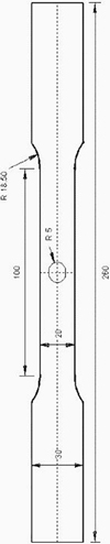 |
Fig. 1 20 × 80 mm tensile specimen with a 10 mm diameter machined hole. |
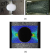 |
Fig. 2 (a) Measurement with binocular microscope. (b) Digital Image Correlation measurement. |
2.1.2 The double-bending specimen
An innovative methodology has been developed at ArcelorMittal for measuring the uniaxial tensile fracture strain. As represented in Figure 3, a bended specimen is bended a second time, perpendicularly to the first direction. This generates a tensile solicitation on the edge.
As illustrated in Figure 4, a strain analysis is performed again using image correlation [5]. However, this method is not adequate on this case due to the speckles deterioration. As shown in Figure 5, failure strain has to be derived from thickness at the vicinity of the crack. Contrarily to the specimen with hole, and because of lower strain gradients, the thickness measurement on a double-bended specimen is accurate enough with a micrometer.
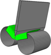 |
Fig. 3 The double bending test: fracture initiates on the machined edge. |
 |
Fig. 4 Image correlation analysis of strain on a double bending specimen. |
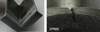 |
Fig. 5 Thickness measurement at the vicinity of the fracture location. |
2.1.3 Comparison between the uniaxial tensile specimen with hole and the double-bending specimen
Fracture strains derived from thickness reduction of both tests presented above are compared for three different steels grades: Dual-Phase 600, Dual-Phase 1180 and Usibor® 1500 (Hot Stamped Steel). Results in Figure 6 highlight that both approaches leading to strain failure under uniaxial tensile load are consistent.
In uniaxial conditions, shortcut is often taken confusing the Uniform Elongation (UEL%), resulting from a standard tensile test, with the ability of grades in terms of fracture strain. This too obvious way to assess the fracture strain is incorrect. For such tensile test specimens, the fracture strain corresponds to the local Reduction of Area (RA) at the failure position. The fracture strain measured in uniaxial tensile strain condition by the local RA could be plotted against the classical UEL% to highlight that there is no direct link between both values. Figure 7 exhibits a large amount of data from numerous grades and thicknesses of the ArcelorMittal automotive product offer. It illustrates clearly that there is no manifest relationship between the UEL% and the fracture strain from RA.
On the other hand, the measurement of the RA value raises the question of uncertainties because there is no easy way to evaluate it as the fracture is rarely in the same plane. Then the double-bending specimen leads to much reliable results of the fracture strain in measuring the thickness reduction more easily.
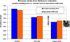 |
Fig. 6 Comparison of tensile failure strain derived from thickness reduction of double bending test and tensile specimen with hole equivalent results. |
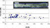 |
Fig. 7 No direct link between Uniform Elongation (UEL%) and failure strain (RA) measured from uniaxial tensile specimen. |
2.2 The equibiaxial expansion test
The fracture strain in equibiaxial expansion is obtained with the Nakajima test [6]; it is described in Figure 8. The homogeneous strain field and low strain rate evolution allow the strain measurement with a Digital Image Correlation analysis (use of VialuxDIC measurement system with a grid of 2 mm [7]). The fracture strain is also derived from thickness reduction at the failure location, i.e. equation (2), assuming isotropic plasticity and equibiaxial strain:
 (2)
(2)
A comparison of the fracture strain obtained by DIC analysis and from thickness reduction has been done for 4 steels grades: DP980LCEY700, DP980Y700, DP1180HY and HR CP800. As illustrated Figure 9, the results are consistent between both methods.
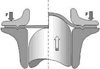 |
Fig. 8 Nakajima test description. |
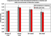 |
Fig. 9 Comparison of the fracture strain in equibiaxial expansion condition is obtained by thickness reduction and DIC analysis. |
2.3 The plane strain test
2.3.1 Notched tensile specimen
As proposed by MatFEM [3], the plane strain path is obtained with a notched tensile specimen. Specimen used at ArcelorMittal is provided Figure 10.
The fracture strain is determined by thickness reduction at the broken cross section, illustrated in Figure 11.
Assuming isotropic plasticity, the local failure strain is directly derived from final and initial thickness ratio, i.e. following equation:
 (3)
(3)
As for the tensile specimen with hole, the advantage of this method is its simplicity, but its drawback is the need of a high precision thickness measurement (microscope).
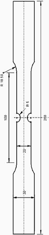 |
Fig. 10 Notched tensile specimen used at ArcelorMittal to measure the fracture strain in plane strain condition. |
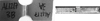 |
Fig. 11 Broken specimen (left) and thickness reduction measured by binocular camera (right). |
2.3.2 The V-bending test VDA-238-100 [8]
As represented in Figure 12, the VDA-238-100V-bending test [8] consists in applying a load on a wide and sharp punch to deflect a small flat specimen supported by two rolling cylinders. This test used in the automotive industry either to assess material ductility or to validate rheological or fracture criteria [9]. It gives the advantage to avoid instability effects. It is moreover quite representative of a fracture caused by a local buckling that could occur in structural parts during a crash event.
The failure strain measurement has to be adapted to this specific test. Due to the strain gradient through the thickness, the fracture strain cannot be derived from final and initial thickness ratio as previously exposed. Nevertheless, Figure 13(a) and (b) shows how the failure strain value can be obtained thanks to DIC analysis (here the GOM ARAMIS system [5]) or finite elements analysis (FEA using ABAQUS [10]). The strain at failure is measured at the extrados of the bending. The imposed displacement in calculation corresponds to the one measured experimentally at the failure occurrence.
Figure 14 shows that the DIC analysis measurement compares with simulation results are in very good agreement, but with the condition that the used meshes are equivalent in terms of size. A mirror was used in order to capture the deformation in the extrados under the tool adding noise on the measure. Moreover, using mesh size much higher than the radius of punch increases oscillations on the measure (calculations over several pixels not in the same plane) and leads to an early loss of signal. In simulation, a 0.2-mm mesh size is fine enough, because convergence is reached.
During a V-bending test, the strain increases smoothly. The exploitation is then more accurate.
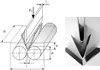 |
Fig. 12 Scheme of the V-bending VDA-238-100 [8] test used at ArcelorMittal and specimen at different bending angle. |
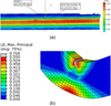 |
Fig. 13 (a) Strain field measured by GOM ARAMIS system at the extrados of the bending. (b) Strain field through the thickness obtained by FEA, fracture strain is taken on the outer skin. |
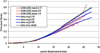 |
Fig. 14 Comparison between measured strains with GOM ARAMIS system and calculated strains in FEA for different mesh size. |
2.3.3 Comparison between the V-bending test and notched specimen tensile test
Figure 15 shows that both tests used to determine the failure strain under a plane strain condition are consistent.
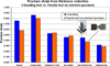 |
Fig. 15 Values of the fracture strain under plane strain obtained with V-bending helped by FEA (blue) and notch tensile tests by thickness measurement (orange). |
3 Synthesis of failure strain measurement
Figure 16 allows the synthesis of failure strains for two dual-phase (DP980 and DP1180) and two press hardened (DUCTIBOR®1300 and USIBOR®1500) steels grades, according to 3 considered strain paths. It provides the equivalent fracture strain according to the stress triaxiality for these grades. The stress triaxiality as well as the equivalent fracture strain is defined further in the present document.
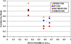 |
Fig. 16 Equivalent failure strain according to the stress triaxiality. |
4 Failure prediction in crash simulation
4.1 Presentation of failure models
As a first approximation the failure risk can be estimated on the basis of the level of plastic strain in the critical area of a component. However, failure models available in LS-DYNA, using more accurate failure criteria based on principal strain or triaxiality, allow obtaining a better failure prediction. The previous experimental data are then used to calibrate different failure models available in LS-DYNA 971 VR4.2.1 & R5.0 [2], such as material laws MAT224, MAT123 [2] and CrachFem model [3].
4.1.1 Failure criterion in MAT123
The MAT123 [2] failure model assumes that the failure occurs at a critical principal strain value, without any dependency on the stress triaxiality. The plane strain condition is assumed to be the most critical strain state for crash applications. Consequently, if the principal failure strain under a plane strain loading is used in this failure criterion, the failure should be roughly estimated. The possibility to use the equivalent strain in the failure calculation was not adopted and is not presented in this paper.
4.1.2 The CrachFEM failure model
The most complete failure model studied in this paper is the CrachFEM model [3]. This model was developed for failure prediction during forming applications and crash. Three failure modes are accounted:
-
normal ductile fracture,
-
shear ductile fracture,
-
instability (necking).
Each failure type is modelled separately and is calibrated regarding specific tests. For crash applications, it is assumed here that mainly the normal ductile failure shall be considered, because necking and ductile shear failures do not occur habitually. The ductile failure model applied to sheet assumes that equivalent failure strain  defined by equation (4) only depends on stress triaxiality η:
 (4)
(4)
And the stress triaxiality is defined by the following equation:
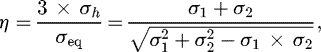 (5)
where η+ is the triaxiality in equibiaxial tension (2 for isotropic plasticity material), η− is the triaxiality in equibiaxial compression (−2 for isotropic plasticity material),
(5)
where η+ is the triaxiality in equibiaxial tension (2 for isotropic plasticity material), η− is the triaxiality in equibiaxial compression (−2 for isotropic plasticity material),  is the equivalent fracture strain in equibiaxial tension,
  is the equivalent fracture strain in equibiaxial compression and c is a parameter taking into account orientation dependency.
Assuming a plane stress state and an isotropic plasticity, the triaxiality η is directly derived from principal strains ε1 and ε2 and more especially by the ratio α between them as defined by the following equation:
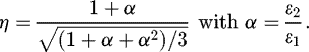 (6)
(6)
The criterion  according to the ratio α is represented in Figure 17.
 ,
,  and c, the model's parameters are calibrated using three experimental results, with α values of three different ratios:
-
the V-bending test or notch specimen tensile test (plane strain state, i.e. α = 0),
-
the Nakajima test (equibiaxial expansion strain state, i.e. α = 1);
-
and the specimen with hole or double bending specimen (uniaxial tensile strain state, i.e. α = −0.5).
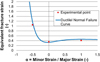 |
Fig. 17 Example of normal ductile fracture curve according to the ratio α. |
4.1.3 The failure model in MAT224
The MAT224 [2] model takes into account the stress triaxility for the fracture strain limit, but it does not make difference between the different failure modes (shear, normal ductile or necking). It could be defined as an intermediate model between the MAT123 [2] and CrachFEM [3] failure models. It represents a good compromise for failure prediction during crash.
The failure curve is defined by several couples of points. In the present case, the same points that the ones used for the Crach FEM model calibration.
4.2 Input parameters of the failure models
Fully integrated shell elements with 5 integration points through the thickness are used to model the specimen. The 3 points bending test consists in applying a load through an impactor having an initial velocity of 8 m/s to deflect a small omega shaped specimen (Fig. 18) made of an AHSS, supported by two cylinders.
Experimentally, it is observed that failure is initiated in the plastic hinge area of the specimen. The simulation is in good agreement with the experimental force-deflection curve (Fig. 18) and the energy absorption capacity (Fig. 19).
Reducing the mesh size of the FE model leads to a higher value of the local strains in the plastic hinge area (Fig. 20). Consequently an accurate failure prediction will require a compensation for the mesh-dependency.
Therefore, simulations with different fixed mesh size are achieved. The principal strain in critical elements is then obtained at the right time and deflection. The regularization curve is then plotted in order to determine the correct failure initiation for different mesh sizes (Fig. 21 for instance with the pink curve). The regularization curve provides the required strain value when the failure should be initiated in order to correlate properly with the experimental crack apparition. The input parameters of the failure models are then calibrated in order to accurately reproduce the crack occurrence. In the present example, the MAT123 failure model is used, being based on the major strain in plane EPSMAJ.
This strain state is the most critical mode of deformation and it corresponds to the lowest point of the fracture curve versus the strain path given Figure 17, i.e. for α = 0. Indeed it can generally be assumed that this strain state, i.e. a plane strain state, is the most critical for crash applications. In Figure 17, failure strain values are taken negative because principal strains are considered. A positive value means that fracture strains are expressed as equivalent values. Then the major strain in plane (EPSMAJ) values for different mesh sizes are obtained from the regularization curve.
It is assumed that failure of an element occurs if one entire layer of its integration points reaches the failure value. Thus, with fully integrated elements and five integration layers, the element is deleted in LS-DYNA if four integration points in the element (NUMINT = 4) reach the single limit strain value (EPSMAJ). An example is provided in Figure 22 with the MAT123 failure model.
The comparison of failure prediction between the experiment results and the FE analyses using MAT123 shows a good correlation for every mesh size. However, fracture strain is depending on the strain path and a failure model based on a single value of major strain in plane EPSMAJ could be insufficient for an accurate failure prediction. Then both MAT224 and CrachFem model allow obtaining relevant failure predictions by using the representation of the equivalent fracture strain according to the strain path (or stress triaxiality). These curves were obtained by the following methodology.
The major in plane strain (EPSMAJ) obtained numerically for every mesh size can be expressed as an equivalent fracture strain versus triaxiality. Then, it becomes possible to compare these values with the experimental values. It was noticed in plane strain condition, that the experimental fracture strain was systematically very close to the calculated equivalent fracture strain for a mesh size of 3 mm (Figs. 20 and 21: 3 mm mesh size at 9 ms). It could be assumed that the experimental values could be directly used as input parameters for a failure model based on equivalent fracture strain, i.e. the MAT224 and CrachFem model with a mesh size of 3 mm. If the regularization curve is available for a particular stress state; it is supposed that the mesh dependency is similar for all strain paths. As illustrated in Figure 23, the equivalent fracture strain (or stress triaxiality) in biaxial expansion and in uniaxial tension is obtained by a simple translation of the experimental values.
By fitting these three values, it is then possible to obtain the curve equivalent fracture strain versus strain path for each mesh size.
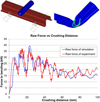 |
Fig. 18 Comparison of force versus deflection curves between FEA and experiments on a 3 points bending test. |
 |
Fig. 19 Comparison of energy absorption capacity between FEA and experiments on a 3 points bending test. |
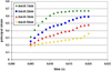 |
Fig. 20 Influence of the mesh size on the principal strain in critical elements of the plastic hinge area. |
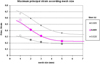 |
Fig. 21 Mesh regularization curve. |
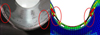 |
Fig. 22 Comparison of failure initiation on a specimen for a 3 mm mesh size using MAT123. |
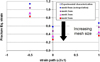 |
Fig. 23 Influence of the mesh size on the equivalent fracture strain versus strain path curve (or triaxiality). |
4.3 Validation of the failure models on a B-pillar
After being calibrated and corrected according to different mesh sizes, the 3 failure models have been applied on a real automotive component. The test consists in impacting in very severe condition a B-pillar made of the press hardened steel grade USIBOR®1500 (thickness 1.8 mm) in order to obtain failures (Fig. 24).
Simulations using the MAT123, MAT224 and CrachFem models are performed on the corresponding B-pillar using FE models for a mesh size of 2 mm, 3 mm and 5 mm. For both MAT123 and MAT224 models, if four integration points in an element (NUMINT = 4) reach the failure criteria then the element is deleted. For the CrachFem model, the element is eliminated if all points of an outer layer of the element reach the critical strain value. These three material models are able to predict the failure in the plastic hinge area for each mesh size which is consistent with the experimental results. Figure 25 provides an illustration with the MAT224 model where the first element deletion time and the number deleted elements are specified.
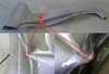 |
Fig. 24 Failure obtained on a very sever impacted of a B-pillar component made of USIBOR®1500. |
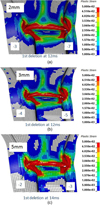 |
Fig. 25 MAT224 failure model applied on a very severe impacted B-pillar made of USIBOR®1500, specification of the number of deleted elements and first element deletion time for (a) 2 mm, (b) 3 mm and (c) 5 mm mesh size. |
5 Conclusions
In this paper, a methodology for the calibration of three different failure models has been proposed. These models are based on the definition of a critical strain leading to failure in the critical area of a considered component. Depending on their complexity, these models can take into account, or not, the stress triaxiality defined by η = 3 × σh/σeq which, in the case of a plane stress state, is equivalent to the strain path defined by α = ε1/ε2.
For this purpose, the failure strains were measured according to three strain states (a uniaxial tensile state, a plane strain state and an equibiaxial strain state). Two innovative ideas were exposed with the use of simple tests: the V-bending test and the double bending test for plane strain and uniaxial tensile states respectively. These tests should lead to a better accuracy of the failure strain measurement, and finally to a better failure prediction. The failure strains of the three investigated failures models have been regularized regarding the effect of the used mesh size.
Finally, the three models were applied on a severely impacted real automotive part, a B-pillar, for three different mesh sizes. The reliability of prediction was demonstrated for all failure models. In this study, the simplest MAT123 failure model was as good as more complex ones as MAT224 and CrachFEM. This is explained by the suitable choice of the failure strain based on the plane strain state condition, assumed to be the most critical and restrictive in crash application. This illustrates that an adequate calibration of the model is a key issue for an accurate failure prediction, more than the choice of the failure model itself.
References
- R. Khamvongsa, A. Bui-Van, D. Cornette, Calibration of fracture parameters and applications for crash simulations of advanced high strength steels, in: ICILLS 2011 (International Conference on Impact Loading of Lightweight Structures, 28th June–1st July 2011), Valenciennes, France, 2011 [Google Scholar]
- LS-DYNA 971/Rev5 (beta) keywords users Manuel, Volume I, Livermore Software Technology Corp., 2010 [Google Scholar]
- H. Dell, H. Gese, G. Oberhofer, CrachFEM: A comprehensive approach for the prediction of sheet metal forming, NUMIFORM'07, in: Materials Processing and Design: Modeling, Simulation and Applications, 18–21st June 2007 [Google Scholar]
- T. Wierzbicki, Y. Bao, Y.-W. Lee, Y. Bai, Calibration and evaluation of seven fracture models, Int. J. Mech. Sci. 47, 719 (2005) [CrossRef] [Google Scholar]
- GOM mbH, ARAMIS – Optical 2015 3D Deformation Analysis, www.gom.com [Google Scholar]
- ISO 12004-2:2008 Metallic materials – Sheet and strip – Determination of forming-limit curves – Part 2: Determination of forming-limit curves in the laboratory [Google Scholar]
- VIALUX AutoGrid®, www.vialux.de [Google Scholar]
- VDA 238-100 Plate bending test for metallic materials, VDA Test Specifications, 2010 [Google Scholar]
- A. Reynes, M. Eriksson, O.-G. Lademo, O.S. Hopperstad, M. Langseth, Assessment of yield and fracture criteria using shear and bending tests, Mater Des. 30, 596 (2009) [Google Scholar]
- ABAQUS, http://www.3ds.com/products-services/simulia/products/abaqus/ [Google Scholar]
Cite this article as: Pascal Dietsch, Kévin Tihay, Antoine Bui-Van, Dominique Cornette, Methodology to assess fracture during crash simulation: fracture strain criteria and their calibration, Metall. Res. Technol. 114, 607 (2017)
All Figures
|
Fig. 1 20 × 80 mm tensile specimen with a 10 mm diameter machined hole. |
| In the text | |
|
Fig. 2 (a) Measurement with binocular microscope. (b) Digital Image Correlation measurement. |
| In the text | |
|
Fig. 3 The double bending test: fracture initiates on the machined edge. |
| In the text | |
|
Fig. 4 Image correlation analysis of strain on a double bending specimen. |
| In the text | |
|
Fig. 5 Thickness measurement at the vicinity of the fracture location. |
| In the text | |
|
Fig. 6 Comparison of tensile failure strain derived from thickness reduction of double bending test and tensile specimen with hole equivalent results. |
| In the text | |
|
Fig. 7 No direct link between Uniform Elongation (UEL%) and failure strain (RA) measured from uniaxial tensile specimen. |
| In the text | |
|
Fig. 8 Nakajima test description. |
| In the text | |
|
Fig. 9 Comparison of the fracture strain in equibiaxial expansion condition is obtained by thickness reduction and DIC analysis. |
| In the text | |
|
Fig. 10 Notched tensile specimen used at ArcelorMittal to measure the fracture strain in plane strain condition. |
| In the text | |
|
Fig. 11 Broken specimen (left) and thickness reduction measured by binocular camera (right). |
| In the text | |
|
Fig. 12 Scheme of the V-bending VDA-238-100 [8] test used at ArcelorMittal and specimen at different bending angle. |
| In the text | |
|
Fig. 13 (a) Strain field measured by GOM ARAMIS system at the extrados of the bending. (b) Strain field through the thickness obtained by FEA, fracture strain is taken on the outer skin. |
| In the text | |
|
Fig. 14 Comparison between measured strains with GOM ARAMIS system and calculated strains in FEA for different mesh size. |
| In the text | |
|
Fig. 15 Values of the fracture strain under plane strain obtained with V-bending helped by FEA (blue) and notch tensile tests by thickness measurement (orange). |
| In the text | |
|
Fig. 16 Equivalent failure strain according to the stress triaxiality. |
| In the text | |
|
Fig. 17 Example of normal ductile fracture curve according to the ratio α. |
| In the text | |
|
Fig. 18 Comparison of force versus deflection curves between FEA and experiments on a 3 points bending test. |
| In the text | |
|
Fig. 19 Comparison of energy absorption capacity between FEA and experiments on a 3 points bending test. |
| In the text | |
|
Fig. 20 Influence of the mesh size on the principal strain in critical elements of the plastic hinge area. |
| In the text | |
|
Fig. 21 Mesh regularization curve. |
| In the text | |
|
Fig. 22 Comparison of failure initiation on a specimen for a 3 mm mesh size using MAT123. |
| In the text | |
|
Fig. 23 Influence of the mesh size on the equivalent fracture strain versus strain path curve (or triaxiality). |
| In the text | |
|
Fig. 24 Failure obtained on a very sever impacted of a B-pillar component made of USIBOR®1500. |
| In the text | |
|
Fig. 25 MAT224 failure model applied on a very severe impacted B-pillar made of USIBOR®1500, specification of the number of deleted elements and first element deletion time for (a) 2 mm, (b) 3 mm and (c) 5 mm mesh size. |
| In the text | |
Current usage metrics show cumulative count of Article Views (full-text article views including HTML views, PDF and ePub downloads, according to the available data) and Abstracts Views on Vision4Press platform.
Data correspond to usage on the plateform after 2015. The current usage metrics is available 48-96 hours after online publication and is updated daily on week days.
Initial download of the metrics may take a while.