© E.I. Castro-Cedeno et al., published by EDP Sciences, 2019

1 Introduction

The treatment of steel in the ladle has become an essential part of the secondary steelmaking process linking primary steelmaking and steel casting. Most secondary steelmaking operations begin with furnace tapping into the ladle and steel deoxidation, followed by adjustment of temperature and chemical composition of the steel, and an inclusion flotation stage before casting. Since endogenous inclusions find their origin as products of steel deoxidation reactions [1], the presence of non-metallic inclusions in the steel is inherent to the deoxidation process itself. In subsequent metallurgical operations, a great deal of effort is invested in reducing the total number of inclusions and controlling the nature of those remaining after steel solidification. For a long time, the gas stirring during ladle treatment has been identified as the processing stage mainly responsible for the control of the inclusion population in steels [2].

As part of the secondary metallurgy practice, calcium is added to certain steel grades with the aim of “modifying” the inclusions in the steel. As a result of the treatment with calcium, alumina and silica inclusions are converted to partially or fully liquid calcium aluminates or calcium silicates [3]. Just like alumina (Al₂O₃), spinel type inclusions (MgO · Al₂O₃) can be modified into liquid inclusions by calcium treatment [4–6]. Before casting, the bath stirring conditions should be controlled to promote inclusion removal by flotation and settling into the slag [7].

The addition of calcium into steel melts is not a trivial problem since this element has a lower density than steel, a low solubility and a great tendency to vaporize at steelmaking temperatures, which typically exceed the normal boiling point of calcium (1757 K) [8]. Special addition techniques such as cored wire injection, schematized in Figure 1, are used for the addition of Ca into liquid steel. The wire consists of a casing tightly wrapped around a core of a Ca-contain material and coiled into a pay-off reel. During injection, the wire is pulled from the reel by a series of pinch rolls of a wire feeding machine and pushed through a guide tube into the steel melt; the casing delays the release of Ca as the wire is injected into the melt and the released time has been predicted by thermal simulation [9].

Regarding the modeling of the calcium treatment of steel with the aims of inclusion modification, several studies have been performed since the 1990s. Lu [10] was one of the first authors to model the kinetics of modification of oxide and sulfide inclusions during the injection of Ca, he acknowledged the effect of S and O contents on the rate of inclusion modification. A follow-up to his work has been recently published [11,12] in which a coupled steel-slag-inclusion kinetic model to estimate the evolution of the bulk composition of the steel and inclusions is presented.

Lately, more computationally costly modeling work has been performed as well. Huang et al. [13] have developed a multi-phase (gas and liquid steel) transient fluid-flow model coupled with the process of injection of the cored wire (i.e. the steel flow is used as input into a model of thermal dissolution of a cored wire). In these simulations, Ca is assumed to be released in gas state. The indicator of mixing efficiency that was considered is the Ca-gas retention rate, however the simulations lack in the sense that no mass transfer with the steel is modelled. Recently, Wang et al. [14] have developed a fluid-flow model in which a set of transport equations for the Ca-vaporization and inclusion modification is solved using the flow state given by the steady-state solution of a two-phase (gas and liquid steel) flow set of equations. The apparent rate for the Ca-vaporization process was fitted by trial and error against experimental data on the evolution of the average Ca concentration in a ladle. By performing thermodynamic calculations, the formation of Al₂O₃, CaO ∙ Al₂O₃, 12CaO ∙ 7Al₂O₃, 3CaO ∙ Al₂O₃, CaS is estimated. Finally, contour plots on the evolution of the different inclusion types are obtained.

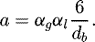
As is also schematized in Figure 1, a Ca particle can be stable as a liquid droplet or a gaseous bubble depending on its position in the ladle. The critical steel depth z_c at which the transition from liquid to gaseous calcium takes place is at the location where the metallostatic pressure p(z) is the same as the calcium vapor pressure P_Ca which is a function of temperature. As an example, the vapor pressures P_Ca at 1823 and 1873 K are 1.36 and 1.77 atm (1 atm = 101325 Pa), corresponding to critical depths in the order of 0.6 and 1.2 m respectively.

The global mass balance for calcium consumption during injection [3] is expressed in equation (1). Once the injected calcium ${{\displaystyle \dot{m}}}_{\mathrm{C}\mathrm{a}\mathrm{,}\mathrm{i}\mathrm{n}\mathrm{j}}$ has been released from the cored wire, the calcium droplets/bubbles ${{\displaystyle \dot{m}}}_{\mathrm{C}\mathrm{a}\mathrm{,}\mathrm{f}\mathrm{r}\mathrm{e}\mathrm{e}}$ dissolve into the liquid steel ${{\displaystyle \dot{m}}}_{\mathrm{C}\mathrm{a}\mathrm{,}\mathrm{d}\mathrm{i}\mathrm{s}\mathrm{s}}$. If Ca is released below the critical depth, the dissolving liquid droplets transform into gas bubbles once they reach the critical depth. Bubbles of calcium undergoing dissolution into the steel eventually reach the free surface of the bath where they either react with the slag ${{\displaystyle \dot{m}}}_{\mathrm{C}\mathrm{a}\mathrm{,}\mathrm{s}\mathrm{l}\mathrm{a}\mathrm{g}}$ or are burnt into the atmosphere ${{\displaystyle \dot{m}}}_{\mathrm{C}\mathrm{a}\mathrm{,}\mathrm{v}\mathrm{a}\mathrm{p}}$. Calcium that has been dissolved into the steel readily reacts with inclusions and modifies them. A part of the inclusions remains in the bath ${{\displaystyle \dot{m}}}_{\mathrm{C}\mathrm{a}\mathrm{,}\mathrm{i}\mathrm{n}\mathrm{c}}$ while the rest are removed from the steel ${{\displaystyle \dot{m}}}_{\mathrm{C}\mathrm{a}\mathrm{,}\mathrm{i}\mathrm{n}\mathrm{c}}^{\text{'}}\text{.}$. $${{\displaystyle \dot{m}}}_{\mathrm{C}\mathrm{a}\mathrm{,}\mathrm{i}\mathrm{n}\mathrm{j}}={{\displaystyle \dot{m}}}_{\mathrm{C}\mathrm{a}\mathrm{,}\mathrm{f}\mathrm{r}\mathrm{e}\mathrm{e}}+{{\displaystyle \dot{m}}}_{\mathrm{C}\mathrm{a}\mathrm{,}\mathrm{d}\mathrm{i}\mathrm{s}\mathrm{s}}+{{\displaystyle \dot{m}}}_{\mathrm{C}\mathrm{a}\mathrm{,}\mathrm{s}\mathrm{l}\mathrm{a}\mathrm{g}}+{{\displaystyle \dot{m}}}_{\mathrm{C}\mathrm{a}\mathrm{,}\mathrm{v}\mathrm{a}\mathrm{p}}+{{\displaystyle \dot{m}}}_{\mathrm{C}\mathrm{a}\mathrm{,}\mathrm{i}\mathrm{n}\mathrm{c}}+{{\displaystyle \dot{m}}}_{\mathrm{C}\mathrm{a}\mathrm{,}\mathrm{i}\mathrm{n}\mathrm{c}}^{\text{'}}\text{.}$$(1)

Since calcium additions during cored wire injection are in the order of several kilograms for an injection time of typically a couple of minutes, the gas evolution caused by the vaporization of Ca effectively modifies the bath stirring conditions. In this work, we simulate the transient fluid-flow and inclusion modification during the Ca-treatment, including the cored wire injection and soft stirring periods. We consider that Ca is released in gas state and that Ca-mass transfer from the gas to the liquid steel occurs before inclusion modification takes place. For the calculation of inclusion modification, the CFD calculations are coupled with thermodynamic calculations performed with the dedicated software CEQCSI, which allows us to estimate the content of calcium-aluminates, spinels and sulfide type inclusions. Hence, one of the objectives of this study is to evaluate qualitatively the extent of the effect of Ca evaporation on the bath stirring by means of fluid-dynamics simulations. The second objective is to gain insight into the process of inclusion modification due to calcium treatment. This numerical work is then an original one since calcium mass transfer is taken into account at the bubble scale, the thermodynamic equilibrium is calculated at each location into the ladle and matter transport is simulated at the scale of the industrial ladle. A particular attention has been paid to the turbulent flow induced by the bubble swarms.

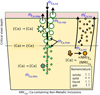Fig. 1 Calcium mass balance during cored injection in the ladle for inclusion modification. Free Ca is stable either as liquid droplet or gaseous bubbles depending on the metallostatic pressure.

2 Methods

A fluid-dynamic model within the framework of the CFD code Ansys Fluent V17.1 was developed in order to simulate the two-phase gas-liquid flow inside a steel ladle using a Euler-Euler approach. The model has previously been described and more detailed information is available in references [15,16]. The CFD calculations are coupled with the thermodynamic software CEQCSI (Chemical EQuilibrium Calculation for the Steel Industry) developed at ArcelorMittal Research in order to estimate the nature of the non-metallic inclusions in the steel as a function of the local steel composition.

2.1 Modeling of the liquid steel-gas mixture

The dispersed phase (gas) is governed by a set of partial differential equations expressing the conservation of mass (Eq. (2)) and momentum (Eq. (3)) similar to the equations applied to the continuous phase (liquid steel). This two-fluid model is expressed as follows: $$\frac{\partial }{\partial \mathit{t}}({\mathit{\alpha }}_{\mathit{k}}{\mathit{\rho }}_{\mathit{k}})+\nabla \cdot ({\mathit{\alpha }}_{\mathit{k}}{\mathit{\rho }}_{\mathit{k}}{\overrightarrow{\mathit{u}}}_{\mathit{k}})=0,$$(2) $$\frac{\partial }{\partial \mathit{t}}({\mathit{\alpha }}_{\mathit{k}}{\mathit{\rho }}_{\mathit{k}}{\overrightarrow{\mathit{u}}}_{\mathit{k}})+\nabla \cdot ({\mathit{\alpha }}_{\mathit{k}}{\mathit{\rho }}_{\mathit{k}}{\overrightarrow{\mathit{u}}}_{\mathit{k}}\otimes {\overrightarrow{\mathit{u}}}_{\mathit{k}})=-{\mathit{\alpha }}_{\mathit{k}}\nabla \mathit{p}+\nabla \cdot ({\mathit{\alpha }}_{\mathit{k}}{\displaystyle \overline{{\displaystyle \overline{\tau }}}})+{\mathit{\alpha }}_{\mathit{k}}{\mathit{\rho }}_{\mathit{k}}\overrightarrow{\mathit{g}}+{\overrightarrow{\mathit{F}}}_{\mathit{k}}\mathrm{.}$$(3)

In the model, the local pressure p is assumed to be shared between the two phases. ${\overrightarrow{\mathit{F}}}_{\mathit{k}}$ represents all the interaction forces between the phases ${\overrightarrow{\mathit{F}}}_{\mathrm{g}}=-{\overrightarrow{\mathit{F}}}_{\mathrm{l}}$ per unit volume, coupling the two sets of equations (for liquid and gas). Four interaction forces are accounted for: drag, lift, added mass effect and turbulent dispersion. The turbulence of the continuous phase is calculated with the standard k − ε model, and for the dispersed phase the turbulent quantities are provided as a function of the results of the continuous phase and the bubble Stokes number. An additional contribution to the liquid effective viscosity is introduced for modeling the turbulence induced by the bubble motion. At the inlet (porous plugs) and outlet (free surface of the bath) of the gas flow, the model incorporates additional source terms in equations (2) and (3) with the aims of modeling the gas injection and the degassing. Concerning the liquid steel phase, a slip condition is applied either at the inlet and outlet surfaces. A large number of user defined functions (UDFs) has been incorporated in order to take into account the specific features of the model [15].

The evolution of the concentration of each chemical species i constituting the continuous and dispersed phases is expressed by a corresponding equation of conservation for the concentration of i in phase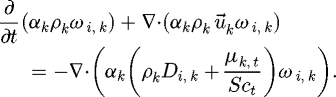: ${\mathit{\omega }}_{\mathit{i}\mathit{,}\mathit{k}}$ (Eq. (4)). $$\frac{\partial }{\partial \mathit{t}}({\mathit{\alpha }}_{\mathit{k}}{\mathit{\rho }}_{\mathit{k}}{\mathit{\omega }}_{\mathit{i}\mathit{,}\mathit{k}})+\nabla \cdot ({\mathit{\alpha }}_{\mathit{k}}{\mathit{\rho }}_{\mathit{k}}{\overrightarrow{\mathit{u}}}_{\mathit{k}}{\mathit{\omega }}_{\mathit{i}\mathit{,}\mathit{k}})=-\nabla \cdot ({\mathit{\alpha }}_{\mathit{k}}({\mathit{\rho }}_{\mathit{k}}{\mathit{D}}_{\mathit{i}\mathit{,}\mathit{k}}+\frac{{\mathit{\mu }}_{\mathit{k}\mathit{,}\mathit{t}}}{{\mathit{S}\mathit{c}}_{\mathit{t}}}){\mathit{\omega }}_{\mathit{i}\mathit{,}\mathit{k}})\mathrm{.}$$(4)

The steel phase is constituted by a mixture of dissolved elements and non-metallic inclusions, all listed in Table 1. The difference of density between non-metallic inclusions and liquid steel is neglected and inclusions are thus transported as tracers inside the steel. It is also considered that the diffusion coefficient is the same for all the constituents of the mixture D_{i, k} = 10^–9 m²s^–1. From this table, it is seen that Ca is present in the liquid steel phase either as a solute element or as a constituent of non-metallic inclusions.

The gas phase is constituted by a mixture of argon and calcium. Ar is the stirring gas introduced through the porous plugs at the bottom of the ladle, while gaseous Ca originates from cored wire injection treatment. Details of the modeling approach for the cored wire injection treatment are given below.

2.2 Modeling of the calcium treatment

2.2.1 Release of calcium into the melt during injection

As a first approach, it is assumed that all injected Ca is released in the gaseous state at the critical depth and at the vertical projection of the position where the cored wire is injected. The dissolution of Ca droplets below the critical depth is neglected. A set of Fluent UDFs has been incorporated in order to take into account the calcium injection process. The mass rate of Ca injection per unit volume at the position of release of Ca, given by equation (5), depends on the wire injection velocity |u_wire| and the linear density of calcium contained in the wire ${\rho }_{\mathrm{C}\mathrm{a}\mathrm{,}\mathrm{w}\mathrm{i}\mathrm{r}\mathrm{e}}$, i. e. the mass of calcium per unit length of wire. 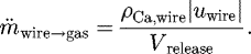$${{\displaystyle \ddot{m}}}_{\mathrm{w}\mathrm{i}\mathrm{r}\mathrm{e}\mathrm{\to }\mathrm{g}\mathrm{a}\mathrm{s}}=\frac{{\rho }_{\mathrm{C}\mathrm{a}\mathrm{,}\mathrm{w}\mathrm{i}\mathrm{r}\mathrm{e}}\left|u_{\text{wire}}\right|}{V_{\text{release}}}\text{.}$$(5)

2.2.2 Calcium interphase mass transfer

Ca bubbles rising through the liquid steel stir the melt and mix with the Ar plume as soon as they become in contact. Calcium in the gas mixture is dissolved to a certain extent into the liquid steel before the bubbles reach the free surface of the bath. Calcium dissolution is implemented by means of a set of UDFs. It is considered that the process of Ca dissolution is governed by interphase mass transfer at the boundary layer between the Ca bubble and liquid steel. The volumetric rate of Ca mass transfer is given by equation (6). $${\mathit{m}}_{\mathrm{g}\to \mathrm{l}}={\mathit{h}}_{\mathrm{l}}\mathit{a}{\mathit{\rho }}_{\mathrm{l}}({\mathit{\omega }}_{\mathrm{C}\mathrm{a},\mathrm{l}}^{*}-{\mathit{\omega }}_{\mathrm{C}\mathrm{a},\mathrm{l}}^{\mathrm{\infty }})\mathrm{.}$$(6)

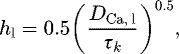
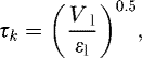
Since the flow inside the ladle is indeed turbulent, Danckwert’s [17] surface-renewal theory seems well appropriate for the calculation of the mass transfer coefficient h_l, because it considers the random renewal of liquid surface around the gas bubble due to the motion of turbulent eddies [18]. Equation (7), derived by Kataoka and Miyauchi [19] and based on Danckwert’s model, assumes that the surface renewal rate corresponds to the smallest eddies and thus is given by the inverse of the Kolmogorov timescale τ_k. It has previously been used by Taniguchi et al. [18] to estimate the gas-liquid mass transfer in gas-injected vessels. The interfacial area of gas-liquid interface per unit volume is calculated with the symmetric model as implemented in Fluent (Eq. (8)), which ensures that the interfacial area concentration approaches zero as α_g approaches one [20]. $${\mathit{h}}_{\mathrm{l}}={0.5(\frac{{\mathit{D}}_{\mathrm{C}\mathrm{a},\mathrm{l}}}{{\mathit{\tau }}_{\mathit{k}}})}^{0.5},$$(7) $${\mathit{\tau }}_{\mathit{k}}={(\frac{{\mathit{V}}_{\mathrm{l}}}{{\mathit{\epsilon }}_{\mathrm{l}}})}^{0.5},$$ $$a={\alpha }_g{\alpha }_l\frac{6}{d_b}\text{.}$$(8)

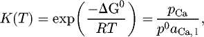
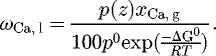
For the calculation of ${\mathit{\omega }}_{\mathrm{C}\mathrm{a},\mathrm{l}}^{*}$, which is the concentration of Ca in the liquid steel in equilibrium with the gaseous Ca in the bubble, the effect of three-phase equilibrium between gaseous calcium, dissolved calcium and inclusions containing Ca is neglected. The only two-phase equilibrium between the gaseous calcium bubble and dissolved calcium in the steel, represented in equation (9), is considered. The corresponding equilibrium constant and free Gibbs energy are given in equations (10) and (11) respectively. $${\text{Ca}}_{\mathrm{g}}\leftrightarrow \left[\text{Ca}\right]\text{,}$$(9) $$\mathit{K}(\mathit{T})=\exp (\frac{-\mathrm{\Delta }{\mathrm{G}}^{\mathrm{0}}}{\mathit{R}\mathit{T}})=\frac{{\mathit{p}}_{\mathrm{C}\mathrm{a}}}{{{\mathit{p}}^0\mathit{a}}_{\mathrm{C}\mathrm{a},\mathrm{l}}},$$(10) $$\mathrm{\Delta }{\mathrm{G}}^{\mathrm{0}}\mathrm{\left[}\mathrm{J}\mathrm{m}\mathrm{o}{\mathrm{l}}^{\mathrm{-}\mathrm{1}}\mathrm{\right]}\mathrm{=}\mathrm{12841}\mathrm{-}\mathrm{51.59}\mathit{T}\mathrm{\left[}\mathit{K}\mathrm{\right]}\mathrm{\text{.}}$$(11)

Equation (12) gives the relation between the activity of calcium in the liquid steel in equilibrium with the partial pressure of Ca in the bubble. Since the model considers that a single pressure is shared by all phases, ${\mathit{p}}_{\mathrm{C}\mathrm{a}}=\mathit{p}(\mathit{z}){\mathit{x}}_{\mathrm{C}\mathrm{a},\mathrm{g}}$. $${\mathit{a}}_{\mathrm{C}\mathrm{a},\mathrm{l}}=\frac{{\mathit{p}}_{\mathrm{C}\mathrm{a}}}{{\mathit{p}}^0\mathit{K}(\mathit{T})}\mathrm{.}$$(12)

In an infinitely diluted Henrian solution, the activity of Ca dissolved in the steel is equal to its concentration. When the 1% mass standard state is used, it follows that: 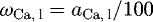${\mathit{\omega }}_{\mathrm{C}\mathrm{a},\mathrm{l}}={\mathit{a}}_{\mathrm{C}\mathrm{a},\mathrm{l}}/100$, hence: $${\mathit{\omega }}_{\mathrm{C}\mathrm{a},\mathrm{l}}=\frac{\mathit{p}(\mathit{z}){\mathit{x}}_{\mathrm{C}\mathrm{a},\mathrm{g}}}{100{\mathit{p}}^0\exp (\frac{-\mathrm{\Delta }{\mathrm{G}}^0}{\mathit{R}\mathit{T}})}\mathrm{.}$$(13)

The second term in equation (6) is the dissolved Ca in the bulk of the liquid bath ${\mathit{\omega }}_{\mathrm{C}\mathrm{a},\mathrm{l}}^{\mathrm{\infty }}$, which is calculated considering that the dissolved elements and non-metallic inclusions in the steel are at local thermodynamic equilibrium. The equilibrium calculations are performed with the thermodynamic software CEQCSI [21]. The mass transfer model is implemented through a set of Fluent UDFs developed for this purpose.

2.3 Coupling of CFD and thermodynamic calculations

The approach for coupling CFD and thermodynamic calculations is similar to that presented in a previous publication [22]: Fluent computes the transport of all dissolved elements and non-metallic inclusions in the liquid steel. Once computation is complete, the data necessary to perform thermodynamic calculations with CEQCSI are transferred, i.e. for each finite volume cell, the contents of dissolved elements and non-metallic inclusions, temperature, pressure. The new distribution of species for each cell is calculated by CEQCSI and transferred back to Fluent, after which the fluid flow calculation is resumed. The coupling between CEQCSI and Fluent is consequently a weak coupling, and is handled through a set of Fluent UDFs. Efforts were pursued to reduce the calculation time of both Fluent and CEQCSI by using parallel computation.

3 Results and discussion

3.1 Industrial trials for model validation

In order to validate the numerical modelling, trials were achieved at an industrial scale in one of the ARCELORMITTAL plants. The typical chemical composition of the steel is listed in Table 2. During two heats, labeled 3191 and 3192, steel samples were taken using an Ar-blown Provac hand lance system before, during and after the wire injection treatment with the aim of observing the evolution of the total calcium content. With this type of device contamination of the sample due to penetration of slag is prevented by Ar blowing through the probe during its introduction into the bath. Moreover, the absence of a metallic cap at the leading edge of the sampler prevents contamination due to mixing of the cap material with the liquid steel. The nomenclature used to identify the steel samples is presented in Table 3 along with the sampling time and the result of the analysis of total calcium by Optical Emision Spectroscopy. The total calcium analysis includes the dissolved calcium and calcium present in inclusions, i.e.: $${\omega }_{\mathrm{C}\mathrm{a}\mathrm{,}\mathrm{t}\mathrm{o}\mathrm{t}}={\omega }_{\mathrm{C}\mathrm{a}\mathrm{,}\mathrm{l}}+{\omega }_{\mathrm{C}\mathrm{a}\mathrm{,}\mathrm{i}\mathrm{n}\mathrm{c}}\text{.}$$

Figure 2 presents schematically a top view of the 190 t industrial ladle where the relative positions of the porous plug, calcium injection and sampling location are shown. The steel samples were taken manually with a Provac hand lance system at a steel depth of approximately 40 cm. To prevent slag from penetrating the sampler, an argon gas flow through the probe is used instead of the metallic cap. This prevents contamination of the steel sample by mixing of the metallic cap material with the liquid metal bath.

Simulations were achieved with the ladle model taking into account the treatment conditions during the industrial trials as operating conditions. Hence, the ladle geometry, steel composition, Ar flow rate in the porous plug, and the Ca injection mass flow rate were all taken from plant data. The industrial practice is to inject calcium for 60 seconds, followed by a long soft-stirring period where the ladle chemical composition is homogenized before sending the heat to the continuous casting machine. In the simulation, the pre-injection ladle flow is initialized by injecting Ar through the porous plug until quasi-steady state is reached. The chemical composition of the steel in the simulation (t = 0) was initialized with the results of the pre-injection steel sample, and considering 5 ppm Ca and 5 ppm Mg.

Figure 3 presents a comparison between the total calcium measured in the steel samples and the calculated average total calcium at the steel sampling point (see Fig. 2). Two values of calcium diffusivity in liquid steel were considered in the simulations, 10⁻⁹m²s⁻¹ and 10⁻⁸m²s⁻¹ which are in the range of the most available data of the literature [10]. The agreement is fairly good for heat 3192, however we can note a discrepancy for the mid-injection sample on heat 3191. This could be explained by the fact that the steel sampling is difficult under the stirring conditions experienced during Ca treatment, thus incertitude with respect to the exact sampling location exists. A careful look at the map of the calcium mass transfer rate calculated by numerical simulation will show (see beyond Fig. 7b) an important gradient in the assumed sampling location. Another reason might be that the model assumes that the wire travels vertically before releasing the calcium. In reality the wire might bend out of trajectory and calcium could be released at a different location than the one prescribed in the simulations, which would lead to variations in the calcium content at the sampling location.

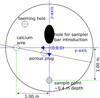Fig. 2 Schematic top view of the ladle showing the position of the porous plug, injection of the cored wire and the sampling of liquid steel.

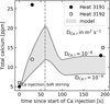Fig. 3 Comparison of measured and computed total calcium content in the steel sample.

3.2 Hydrodynamics during calcium injection

As an example of the typical fluid flow present during Ca injection, Figure 4 gives the computed gas retention (Fig. 4a) and the liquid steel velocity vectors (Fig. 4b) in the plane crossing the calcium injection point and the porous plug. Furthermore, Figure 5 draws maps of the turbulent kinetic energy (Fig. 5a) and its dissipation rate (Fig. 5b). In all the figures, the 1% volume gas fraction delimiting the shape of the plume (thin magenta or gray line) and the locations of the release of Ar (porous plug) and Ca gas are identified as well.

Naturally, the mushroom shaped gas plume has higher gas retention in the zones near the porous plug and close to the calcium release (Fig. 4a). The steel velocity vectors (Fig. 4b) show that there is a continuous feeding of fresh steel into a highly turbulent zone (Figs. 5a and 5b) where Ca is released. The Ca-enriched steel is afterwards transported away from this turbulent region into zones far away from the plume where steel velocities and turbulence are reduced. The lowest value of the Kolmogorov scale (20 µm) is reached in the highly turbulent region.

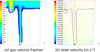Fig. 4 (a) gas volume fraction; (b) steel velocity vectors at mid-injection (t = 30 s). The total Ca injection time was of 60 s.

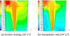Fig. 5 (a) contours of turbulent kinetic energy; (b) dissipation rate at mid-injection (t = 30 s).

3.3 Hydrodynamics after calcium injection

Similar maps of gas retention and steel velocities are drawn in Figures 6a and 6b after Ca injection (t = 200 s). Once the Ca injection has been stopped (t = 60 s), the plume shrinks from the spreading mushroom shape seen in Figure 4a to the rising plume shape seen in Figure 6a. During the transient plume shrinking period (around 40 seconds) Ca is still transferred from the gas phase to the liquid steel before the Ca gas is released on the surface. At the end of this transient period, the rising plume is constituted of pure Ar. The steel velocity vectors (Fig. 6a) emphasize the steel recirculation zones surrounding the rising gas plume, and as a consequence the smallest velocities are found at the bottom of the ladle. The averaged steel and gas velocities inside gas plume are equal to 0.6 and 0.8 m/s respectively, these values agree well with numerical data calculated by CFD by Lou and Zhu for an industrial scale ladle [23].

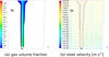Fig. 6 Gas volume fraction and steel velocity vectors at post-injection (t = 200 s). The total Ca injection time was of 60 s.

3.4 Calcium mass transfer

Figure 7 presents contours of the chemical composition of the plume and the volumetric Ca mass transfer rate in the gas phase. The plume can be split into three zones based on its composition (Fig 7a): the tail constituted by the Ar coming from the porous plug, a Ca-rich region near the zone of release of Ca and an Ar-Ca mixing zone far away from it. It is in the Ca-zone that indeed Ca mass transfer is maximized (Fig. 7b). According to the mass transfer equation (Eq. (6)), the transfer is maximized when the product of the volumetric mass transfer coefficient h_la and the chemical potential 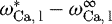${\mathit{\omega }}_{\mathrm{C}\mathrm{a},\mathrm{l}}^{*}-{\mathit{\omega }}_{\mathrm{C}\mathrm{a},\mathrm{l}}^{\mathrm{\infty }}$ increases. From the models chosen for the calculation of h_l (Eq. (7)) and a (Eq. (8)), h_la is enhanced in high turbulent zones (Fig. 5b) where the volume fraction of gas ${\mathit{\alpha }}_{\mathrm{g}}$ approaches a value of 0.5 (Fig. 4a). On the other hand, the potential term is optimized in zones where the gas is rich in Ca, i.e. the term ${\mathit{\omega }}_{\mathrm{C}\mathrm{a},\mathrm{l}}^{*}$ (calculated by means of Eq. (13)) attains its maximum when the molar fraction of Ca in the gas ${\mathit{x}}_{\mathrm{C}\mathrm{a},\mathrm{g}}$ is equal to one (Fig. 7a).

The degree of Ca mixing in the ladle is deduced from the contours of the local total calcium content in the steel shown in Figure 8. At the end of Ca injection (t = 60 s), the liquid steel that has already been enriched with Ca is mostly found above mid-height in the ladle (Fig. 8a). This is due to the relatively weak flow far away from the Ca-rich zone of the plume. The gradients of Ca content are progressively reduced during the soft stirring period (Figs. 8b and 8c), and a little over two minutes after the end of injection the steel bath is close to complete homogenization. This time agrees well with the typical mixing time of an industrial ladle measured by Bellot et al. [16].

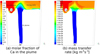Fig. 7 Contours of (a) molar fraction of calcium in the gas and volumetric and of (b) Ca mass transfer rate at mid-injection time (t = 30 s).

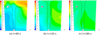Fig. 8 Contours of local total Ca content [ppm].

3.5 Inclusion modification

The coupling between the CFD and thermodynamic codes provides a huge number of data which have been split into global content (averaged value over the molten steel) and maps of local values.

Figures 9a and 9b show the evolution of the inclusion content at the steel sampling position and the global inclusion content obtained in the simulations. The predicted inclusion contents obtained after homogenization match well with the estimated values from sample measurements when low oxygen contents (5 and 10 ppm) are used in the input for the thermodynamic calculations (the measured total oxygen content is 5 ppm before the start of Ca injection). However, we notice a poorer agreement during calcium injection.

The global process of inclusion modification is shown in Figure 9c, and the consecutive inclusion maps in Figure 10 illustrate the evolution of the partition between solid and liquid inclusions during the soft stirring period for the two total oxygen conditions.

Numerical simulations show that solid inclusions are constituted of more than 99% spinel, and liquid inclusions are Ca aluminates with varying degrees of MgO spanning from 1.3 to 6.6 wt.%. As the steel is continuously enriched in Ca during the injection period, there is a rapid increase in the fraction of liquid inclusions (Fig. 8c). During the soft stirring period, the rate of inclusion modification depends on the mixing in the ladle. The zones containing 100% liquid inclusions are those in which the total calcium content (Fig. 7) is greater or equal to the minimum requirement established by steel-inclusion thermodynamic equilibrium. Once the steel is homogenized, the inclusions will be completely liquid.

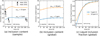Fig. 9 Evolution of the simulated inclusion content in the steel as a function of the total oxygen content. Whiskers in Figure (a) report measured values.

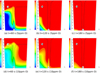Fig 10 Maps of the fraction of liquid inclusions as a function of the total oxygen content (5 or 10 ppm).

4 Conclusions

A numerical tool, based on the coupling between the CFD code ANSYS Fluent and the thermodynamic code CEQCSI, has been developed and applied to industrial configurations in order to investigate the possible effects of the calcium injection practice on the modification of non-metallic inclusions. As a first approach, the inclusion modification by calcium injection treatment can be described rather satisfactorily with simplified assumptions regarding the mechanism of dissolution of calcium into the liquid steel and considering that local thermodynamic equilibrium prevails at all times. However, improvements of the model are possible if a more accurate simulation of the complex behavior of inclusion population is desired. Of course, among those improvements, consideration of the actual kinetics of the inclusion modification process, account of inclusion removal by settling or flotation into the slag [24], and a more realistic description of the top slag layer most likely represent the greatest issues [25]. To do this special interface tracking methods and mesh refining would for sure be needed but leading to an increase of the calculation cost.

From an industrial point of view, the prospective of this work is considerable: the coupling could be applied to different ladle geometries, steel compositions, gas stirring and various injection practices.

Nomenclature

Symbols

a: Interfacial area per unit volume [m⁻¹]

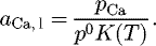
a_Ca,l: Activity of calcium in the steel in equilibrium with Ca bubble [ ]

D_i,k: Diffusivity of species i in phase k [m² s⁻¹]

d_b: Bubble diameter [m]

g: Gravity acceleration [m s⁻²]

h_l: Mass transfer coefficient [m ^s−1]

K(T): Equilibrium constant [ ]

k: Turbulent kinetic energy [m2 s⁻²]

${{\displaystyle \dot{m}}}_{\mathrm{C}\mathrm{a}}$: Global rate of calcium transfer [kg s⁻¹]

${{\displaystyle \ddot{m}}}_{\mathrm{g}\to \mathrm{l}}$: Volumetric mass transfer rate [kg m⁻³ s⁻¹]

${{\displaystyle \ddot{m}}}_{\mathrm{w}\mathrm{i}\mathrm{r}\mathrm{e}\mathrm{\to }\mathrm{g}\mathrm{a}\mathrm{s}}$: Volumetric calcium release rate [kg m⁻³ s⁻¹]

p: Pressure [Pa]

p⁰: Reference pressure (1 atm) [Pa]

p_Ca: Calcium vapor pressure [Pa]

p(z): Metallostatic pressure [Pa]

R: Ideal gas constant, 8.314 [J mol⁻¹ K⁻¹]

Sc_t: Turbulent Schmidt number, = 0.7

t: Time [s]

u: Velocity [m s⁻¹]

u_wire: Wire injection velocity [m s⁻¹]

V_release: Volume of steel where Ca is released [m³]

T: Temperature [K]

t: Time [s]

x_{Ca, g}: Mole fraction of Ca in gas [ ]

z: Depth in the molten steel [m]

Greek Symbols

α: Volume fraction [ ]

$\mathrm{\Delta }{\mathrm{G}}^{\mathrm{0}}$: Standard Gibbs free energy [J mol⁻¹]

ϵ: Turbulent kinetic energy dissipation rate [m² s⁻³]

μ: Dynamic viscosity [Pa s]

v: Kinematic viscosity [m² s⁻¹]

ρ: density [kg m−3]

${\rho }_{\mathrm{C}\mathrm{a}\mathrm{,}\mathrm{w}\mathrm{i}\mathrm{r}\mathrm{e}}$: Wire linear Ca density [kg m−1]

${\displaystyle \overline{{\displaystyle \overline{\tau }}}}$: Viscous stress tensor [Pa]

τ_k: Kolmogorov timescale [s]

ω_i,k: Mass fraction of species i in phase k [ ]

Subscripts

c: Critical

diss: Dissolved

g: Gas

i: Chemical species i

inc: Inclusion

k: Phase k

l: Liquid

slag: Slag

surf: Surface

vap: Vaporized

t: Turbulent

tot: Total

wire: Wire

References

All Tables

All Figures

	Fig. 1 Calcium mass balance during cored injection in the ladle for inclusion modification. Free Ca is stable either as liquid droplet or gaseous bubbles depending on the metallostatic pressure.
In the text

	Fig. 2 Schematic top view of the ladle showing the position of the porous plug, injection of the cored wire and the sampling of liquid steel.
In the text

	Fig. 3 Comparison of measured and computed total calcium content in the steel sample.
In the text

	Fig. 4 (a) gas volume fraction; (b) steel velocity vectors at mid-injection (t = 30 s). The total Ca injection time was of 60 s.
In the text

	Fig. 5 (a) contours of turbulent kinetic energy; (b) dissipation rate at mid-injection (t = 30 s).
In the text

	Fig. 6 Gas volume fraction and steel velocity vectors at post-injection (t = 200 s). The total Ca injection time was of 60 s.
In the text

	Fig. 7 Contours of (a) molar fraction of calcium in the gas and volumetric and of (b) Ca mass transfer rate at mid-injection time (t = 30 s).
In the text

	Fig. 8 Contours of local total Ca content [ppm].
In the text

	Fig. 9 Evolution of the simulated inclusion content in the steel as a function of the total oxygen content. Whiskers in Figure (a) report measured values.
In the text

	Fig 10 Maps of the fraction of liquid inclusions as a function of the total oxygen content (5 or 10 ppm).
In the text

References

- E.T. Turkdogan, R.J. Fruehan, Fundamentals of iron and steelmaking, in R.J. Fruehan (Ed.), The making, shaping and treating of steel: Steelmaking and refining volume, 11th ed., The AISE Steel Foundation, 1998, pp. 13–157 [Google Scholar]
- L. Zhang, B.G. Thomas, State of the art in evaluation and control of steel cleanliness, ISIJ Int. 4(3), 271–291 (2003) [CrossRef] [EDP Sciences] [Google Scholar]
- G.J.W. Kor, P.C. Glaws, Ladle refining and vacuum degassing, in: R.J. Fruehan (Ed.), The making, shaping and treating of steel: Steelmaking and refining volume, 11th ed., The AISE Steel Foundation, 1998, pp. 359–426 [Google Scholar]
- E.B. Pretorius, H.G. Oltmann, T. Cash, The effective modification of spinel inclusions by Ca treatment in LCAK steel, Iron Steel Technol. 7(7), 31–44 (2010) [Google Scholar]
- N. Verma, P.C. Pistorius, R.J. Fruehan, M.S. Potter, H.G. Oltmann, E.B. Pretorius, Calcium modification of spinel inclusions in aluminum-killed steel: Reaction steps, Metall. Mater. Trans. B 43(4), 830–840 (2012) [CrossRef] [Google Scholar]
- E.I. Castro-Cedeno, M. Herrera-Trejo, M. Castro-Roman, F. Castro-Uresti, M. Lopez-Cornejo, Evaluation of steel cleanliness in a steel deoxidized using Al, Metall. Mater. Trans. B 47(3), 1613–1625 (2016) [Google Scholar]
- B.H. Reis, W.V. Bielefeldt, A.C. Faria-Vilela, Absorption of non-metallic inclusions by steelmaking slags – A review, J. Mater. Res. Technol. 3(2), 179–185 (2014) [CrossRef] [Google Scholar]
- T. Ototani, Calcium clean steel, Springer-Verlag, Berlin, 1986 [CrossRef] [Google Scholar]
- E.I. Castro-Cedeno, A. Jardy, A. Carre, S. Gerardin, J.-P. Bellot, Thermal modelling of the injection of standard and thermally insulated cored wire, Metall. Mater. Trans. B 48(6), 3316–3328 (2017) [CrossRef] [Google Scholar]
- D. Lu, Kinetics, Mechanisms and modeling of calcium treatment of steel, PhD thesis, McMaster University, Ontario, 1992 [Google Scholar]
- Y. Tabatabaei, K.-S. Coley, G.-A. Irons, S. Sun, A multilayer model for alumina inclusion transformation by calcium in the ladle furnace, Metall. Mater. Trans. B 49, 375–387 (2018) [CrossRef] [Google Scholar]
- Y. Tabatabaei, K.-S. Coley, G.-A. Irons, S. Sun, Model of inclusion evolution during calcium treatment in the ladle furnace, Metall. Mater. Trans. B 49, 2022–2037 (2018) [CrossRef] [Google Scholar]
- H.-g. Huang, M. Yan, J.-n. Sun, F.-s. Du, Heat transfer of calcium cored wires and CFD simulation on flow and mixing efficiency in the argon-stirred ladle, Ironmak. Steelmak. 45(7), 626–634 (2017) [CrossRef] [Google Scholar]
- S. Wang, J. Zhang, R. Cheng, H. Ma, Numerical simulation of inclusion modification during calcium treatment process in ladle, Trans. Indian Inst. Met. 71(9), 2231–2242 (2018) [CrossRef] [Google Scholar]
- V. De-Felice, I.L. Alves-Daoud, B. Dussoubs, A. Jardy, J.P. Bellot, Numerical modelling of inclusion behaviour in a gas-stirred ladle, ISIJ Int. 52(7), 1273–1280 (2012) [CrossRef] [Google Scholar]
- J.P. Bellot, V. De-Felice, B. Dussoubs, A. Jardy, S. Hans, Coupling of CFD and PBE calculations to simulate the behavior of an inclusion population in a gas-stirring ladle, Metall. Mater. Trans. B 45(1), 13–21 (2014) [CrossRef] [Google Scholar]
- P.V. Danckwerts, Significance of liquid-film coefficients in gas absorption, Ind. Eng. Chem. 43(6), 1460–1467 (1951) [Google Scholar]
- S. Taniguchi, S. Kawaguchi, A. Kikuchi, Fluid flow and gas-liquid mass transfer in gas-injected vessels, Appl. Math. Model. 26(2), 249–262 (2002) [Google Scholar]
- H. Kataoka, T. Miyauchi, Gas absorption into free liquid surface of water tunnel in turbulent region, Kagaku Kogaku 33(2), 181–186 (1969) [CrossRef] [Google Scholar]
- Ansys Fluent 17.0 Theory Guide, Ansys Inc., 2016, pp. 485–628 [Google Scholar]
- J. Lehmann, Applications of ArcelorMittal Maizières thermodynamic models to liquid steel elaboration, Rev. Métall.-Int. J. Metall. 105(11), 539–550 (2008) [CrossRef] [Google Scholar]
- M. Simonnet, J.F. Domgin, J. Lehmann, P. Gardin, Numerical tool coupling fluid dynamics and thermochemistry to predict and to optimize deoxidation processes, BHM Berg-u. Hüttenmänn. Monatsh. 152(11), 350–354 (2007) [CrossRef] [Google Scholar]
- W. Lu, M. Zhu, Numerical simulations of inclusion behavior in gas-stirred ladles, Metall. Mater. Trans. B 44(3), 762–782 (2013) [CrossRef] [Google Scholar]
- J.-P. Bellot, J.-S. Kroll-Rabotin, M. Gisselbrecht, M. Joishi, A. Saxena, S. Sanders, A. Jardy, Toward better control of inclusion cleanliness in a gas stirred ladle using multiscale numerical modelling, Materials 11, 1179 (2018) [CrossRef] [Google Scholar]
- L. Li, B. LI, Z. LIU, Modeling of gas-steel-slag three-phase flow in ladle metallurgy: Part II. Multi-scale mathematical model, ISIJ Int. 57(11), 1980–1989 (2017) [CrossRef] [Google Scholar]
Cite this article as: E.I. Castro-Cedeno, A. Jardy, B. Boissiere, J. Lehmann, P. Gardin, A. Carré, S. Gerardin, Jean-Pierre Bellot, Numerical simulation of modification of non-metallic inclusions by calcium treatment in the argon-stirred ladle, Metall. Res. Technol. 116, 515 (2019)