| Issue |
Metall. Res. Technol.
Volume 120, Number 1, 2023
|
|
|---|---|---|
| Article Number | 117 | |
| Number of page(s) | 16 | |
| DOI | https://doi.org/10.1051/metal/2022094 | |
| Published online | 22 February 2023 | |
Regular Article
Analysis of the microstructural features of phase transformation during hardening processes of 3 martensitic stainless steels
1
LSPM − CNRS, Université Paris 13, 99, av. J.B. Clément, 93430 Villetaneuse, France
2
Laboratoire Quartz (EA 7393), ISAE-Supméca, 3 Rue Fernand Hainaut, 93400 Saint Ouen, France
* e-mail: This email address is being protected from spambots. You need JavaScript enabled to view it.
Received:
11
July
2022
Accepted:
13
October
2022
Abstract
The present paper investigates the microstructural features and associated hardening state of three different martensitic stainless steels (CX13, XD15 and MLX17 produced by Aubert&Duval), subjected to three different thermomechanical treatments, aimed at producing hard materials for tribological applications. It is thus shown that all treatments (cementation, HF quenching or Age Hardening) are efficient to produce hard surfaces. The bulk martensitic state is also studied. Although the three martensites look somewhat different, it is shown that the transformation always obeys the KS orientation relationship with some variant selection, which produces a significant amount of twin boundaries. These results are quite different from those found in low C steels. Based on a quantitative analysis of the EBSD microstructures, a quantification of the various relative hardening contributions (phase transformation, grain size, dislocation density, solid solution effect or precipitation) is then proposed.
Key words: Martensitic stainless steels / electron backscattering diffraction (EBSD) / hardness / phase transformation
© T. Santos et al., Published by EDP Sciences, 2023
 This is an Open Access article distributed under the terms of the Creative Commons Attribution License (https://creativecommons.org/licenses/by/4.0/), which permits unrestricted use, distribution, and reproduction in any medium, provided the original work is properly cited.
1 Introduction
The development of stainless steels for aeronautic combined applications such as high mechanical volume performances (strength, fracture toughness, resilience) and surface performances (friction coefficient and wear rate) represent a major engineering challenge, since many components in this domain operate under severe conditions which can be beyond the material capacities. For example, bearings on engine shafts and gears have to be able to stand vibratory stresses during long periods, high rotation speeds (up to. 25,000 rpm), elevated temperatures and aggressive chemical environments. This is why some thermo-(chemical) treatments, often coupled with additional surfaces treatments, have been developed in order to improve the general mechanical resistance of these materials together with their tribological properties. Among them, two main types of treatments are widely used, namely:
Classical heat treatments, such as age hardening [1], also known as precipitation hardening, which makes use of solid impurities or precipitates for the strengthening process. The alloy is aged by heat treatment, either at high or low temperature, so that precipitates can be formed. In the case of stainless steels, the general process also involves quenching from austenite to martensite which further hardens the material; the final state is thus composed of martensite and precipitates within its whole volume and the surface properties are not different from the core ones; in order to further improve the surface properties, some additional surface treatment such as. ion implantation can be further applied [2].
Thermochemical treatments, such as carburizing [3], which mainly harden the materials within a more or less thick surface layer. It consists in the incorporation of carbon at the surface of low carbon steels within the austenitic range. As a result, carbides are produced within a thick layer at the surface of the material, leading to a gradual increase of the superficial hardness. Case hardening is then achieved again by quenching the material to form a martensitic structure; as a result, the material is formed of (i) martensite plus precipitates in the superficial layer and (ii) and simple martensite in the core of the sample. This type of treatment thus produces a material with an overall improved high yield strength in the core of the material combined with an improved wear and fatigue resistance [4–6].
In between, some more local thermal treatments are also often used, such as e.g. High Frequency Induction Quenching [7,8], in which the metal undergoes a local heating and quenching treatment within the external layer of the material, creating thus a hard martensite at the surface of the material. In that case, no additional component is added to the metal, but the treatment can also lead to some precipitation of the alloying elements of the steel.
These three types of treatments are commonly industrially used to produce hard (or even ultra-hard [9]) martensitic stainless steels especially for tribological applications. Obviously, they mainly differ by the actual thickness within which the material is significantly reinforced by additional superficial treatments, and some recent publications report data concerning the relative contribution of different mechanisms to the overall hardening, both on the surface and in the core of the material (e.g. [9–11]). However, the transformation mechanisms and microstructures are poorly documented in these steels, in spite of the obvious link between microstructural features and mechanical properties. Indeed, the microstructural features, which result directly from the martensitic transformation and that can play a significant role on mechanical strength, are the orientation and misorientation distributions [12], the grain or subgrain (or lath) size and shapes [13] and the distribution of various phases (including the possible distribution of precipitates or of another minor phase inside the grains or along the existing grain boundaries). The result is that, for example, the misorientation profiles, which directly affect the hardening contribution of various types of grain boundaries and which are widely documented in other types of steels [14–17], are sometimes transposed without verification [9], which induces an imprecision on the contribution to the hardening of the grain boundaries.
As all types of above listed thermo-(chemical) treatments imply a martensitic transformation, it may thus be of interest to investigate their influence on both surface and volume microstructures, and the possible link with the overall mechanical and tribological properties [18]. If a 100% martensitic structure is expected within the bulk of the material, it is quite usual to also observe some residual austenite (which, depending on the exact concentration, may alter the hardness of the material) at the surface of the material or sometimes bainite (if quenching is not fast enough) within the interior of quenched samples.
Especially, for the three complex treatments studied in the present work (carburizing, age hardening or HF quenching), the final surface and bulk microstructures will be the consequence of several competing mechanisms such as precipitation, recrystallization, diffusive or displacive phase transformation occurring with or without a so-called variant selection [15,19,20]; these microstructures will strongly influence in turn the anisotropy of the final physical and mechanical properties of the steel [21], and especially the orientation distribution which is a direct consequence of a possible variant selection, or the type, number and distributions of grain boundaries (GB) present in the material, which also have a major influence on e.g. fracture phenomena [22–25].
The purpose of this work is thus to characterize the microstructures formed in three different martensitic stainless steels after three different industrial hardening treatments, to deduce some characteristics of the observed transformation (to see especially if we do observe some orientation relationship between austenitic and martensitic phases and some associated variant selection) and to correlate these observations with the hardness distribution measured through the thickness of the materials. The outline of the present paper is thus as follows: the investigated materials, thermochemical treatments and main characterization techniques are first described in Section 2, the experimental results (microstructures and hardness) are then presented in Section 3 and the so obtained bulk martensitic microstructures are then analyzed in more details in Section 4. A connection with possible hardening mechanisms is presented in Section 5. These data allow to extract the main features of the studied microstructures (in connection with the applied treatment), which are recalled in Section 6 as general conclusions.
2 Material and methods
The investigated materials used in this work are three high strength stainless steels, supplied by Aubert&Duval, whose commercial designations and compositions are presented in Table 1. Additionally, the 3 steels are also designated by the thermomechanical treatment they undergo. All three materials are supplied in the form of disks of diameter 60 mm and a thickness of 6 mm. CS and HFQS alloys have been provided before and after treatment whereas the AHS alloy was provided only in the age − hardened state.
The cemented steel (CX13) is initially supplied in annealed state, being thus entirely composed of bainite. Some samples are then submitted to an industrial thermochemical treatment, consisting of a carburizing step in a low-pressure furnace at a temperature between 900 and 980°C which allows C diffusion on a thickness of several millimeters, followed by homogenization in the austenitic range, oil quenching for martensitic transformation, cold treatment in liquid nitrogen to allow the transformation of the residual austenite into martensite, and a final tempering step for stress release. The HF quenched steel (XD15) is also supplied in an annealed state, being composed of ferrite. Some samples are then submitted to a 2 steps treatment; (i) austenitization above 1000 °C followed by quenching for martensitic transformation and double tempering at 650 °C for softening and stress release and (ii) local induction heating above 1100 °C followed by quenching for martensitic transformation, cold treatment in liquid nitrogen to also transform the residual austenite and a final tempering step at low temperature (below 200 °C) for stress release. As for the age hardened steel (MLX17), the thermal treatment is classically composed of homogenization in the austenitic range, oil quenching, cold treatment in liquid nitrogen and a final tempering step around 500 °C. For this last material, the initial state before AH treatment is not documented. All proposed treatments have been especially designed to allow the martensitic transformation combined with additional hardening mechanisms taking place during the tempering process.
Some smaller parallelepipedic samples (with dimensions 3 mm × 3 mm × 0.5 mm thickness) were then cut from the surface of the large disks (to include the external treated surface) using a Struers Secotom15 cutting machine. Cutting was then followed by mechanical grinding and polishing with a diamond solution up to 1 μm on the transverse section, in order to perform through thickness hardness measurements (with a Buehler instrument using a diamond Vickers (HV0.05) indenter). The samples were then additionally polished with Oxide Polishing Suspension (OPS) in order to perform SEM observations. A Zeiss Supra 40VP SEM equipped with a field emission gun (FEG-SEM) and an integrated Nordif UF 300 detector has been used to perform Electron Back Scattering Diffraction (EBSD). The Kikuchi patterns have been recorded at an accelerating voltage of 20 kV, a specimen tilt angle of 70° and with a step size varying between 100 and 200 nm with the TSL OIM® Data Collection software. The data processing of the raw data was then performed using the TSL OIM® Analysis 7 software, especially to get information regarding the density and nature of the boundaries in the microstructure for these conditions. During the data processing, the data points that have a size less than 2 pixels were cleaned up using the grain dilation method provided in the software (with a tolerance misorientation angle of 5°).
Initial chemical composition of the studied materials (wt.%).
3 Experimental results
3.1 Initial microstructural state before hardening
The microstructures of the CS and HFQS materials before hardening treatment are presented in Figure 1. The microstructural and mechanical characterization of this initial state aims to better understand and quantify the influence of the hardening treatments performed, as well as the efficiency of the martensitic transformation. For the CS material (a), this annealed state has a lath-type structure, typical of bainite formed within these steels [22,26]. The boundaries associated with misorientations between 25° and 45° have been plotted as black lines on the orientation map. Indeed, it is well known that most boundaries between bainite or martensite laths have either low (<25°) or high misorientations (>45°) − see Section 4 – and hence are not visible here [27]. On the contrary, most boundaries that correspond to the prior austenite grain structure are expected to have more or less random misorientations (thus, with a peak around 40°). The resulting GB map is therefore dominated by the prior austenite grain boundaries and so gives a good indication (although not a perfect one, since it is clear that a lot of these grain boundaries are not closed) of the prior austenite grain structure. We can thus conclude that the prior austenitic grain size, just before transformation was equal to 40 μm approximately. Then, the classical subdivision of bainitic grains into laths, grouped into bocks, grouped themselves into packets is also clearly present [28]. This bainite also contains some nanoprecipitates, which cannot be determined by EBSD and are thus not seen on the OIM map, even when only the Image Quality (IQ) index is represented (see Fig. 2a). These have been determined elsewhere [29], and have been shown to be of the type M7C3 (with M = F, Cr, Mo, V) with an average size of 5 nm. If these nanoprecipitates may contribute to the hardening of the material, they also involve a decrease of the resistance to corrosion, since the Cr percentage within the matrix may have decreased.
For the HFQS material, the initial state is supposed to be composed of 100% ferrite. Indeed, the microstructure appears quite different from bainite, and looks indeed closer to a classical recrystallized ferritic microstructure. The represented GBs are not associated with lath packets anymore, and are thus less clearly associated with the prior austenite GBs. In Figure 1b, some black points are also visible which correspond in this case to non-indexed points. We assumed that these points were precipitates. When the orientation is replaced by the image quality (IQ) index for each point, we do see some black points on the map (see Fig. 2b), which indeed look like precipitates. Again, this have been confirmed elsewhere [30] and those precipitates identified as precipitates of the type M23C6 with M = (Cr, Fe, Mo), Cr2N and V2N. The size of these precipitates is much larger than those present in the bainite, and typically around 0.7 μm in average. Again, they may contribute to hardening of the material. Such large precipitates are not visible in the IQ map of the CS material (Fig. 2a).
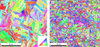 |
Fig. 1 EBSD orientation maps of the CS (a) and HFQS (b) materials determined before hardening treatment. The microstructure is bainitic for the CS steel (a) and ferritic for the HFQS steel (b). The color corresponds to the crystallographic orientation of the ND direction within the crystal reference frame, according to the color code given by the unit triangle. For both microstructures, the step size is equal to 0.2 μm and the boundaries corresponding to misorientations between 25° and 45° have been plotted as dark lines. |
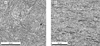 |
Fig. 2 Image Quality (IQ) Index maps of the CS (a) and HFQS (b) materials determined before hardening treatment. |
3.2 EBSD qualitative measurements after hardening treatment
EBSD analysis was then performed for the three steels after hardening treatment in two different zones: the surface (high hardness zone for 2 out of the 3 investigated steels) and the bulk (constant hardness zone) ones. For the AHS material, it was thus verified that the material was homogeneous from the surface to the core. All maps were established from the measured Kikuchi patterns, by considering that the material could be dual phase only (bcc martensite + fcc austenite). The various possible precipitates have been excluded from this analysis, since the number of possibilities would have been too large for the analysis to converge. It is also worth noting that the presence of a very hard phase within the material involves some difficulties in the preparation of the samples. As a result, the quality of the surface maps is lower than that of the bulk measurements and the precipitates are only visible through e.g., differences in Image Quality (IQ) or Confidence Index (CI). Typical surface EBSD maps, both in Image Quality (IQ) and orientation are presented in Figure 3 for the CS and HFQS materials.
For the CS material, the analysis of these maps first indicates that the surface material contains more than 15% of austenite. On the surface maps, the black points correspond to non-indexed points, which have been identified elsewhere as micrometric intra- and inter-granular carbides of the type M23C6 and M7C3 (where M = Cr, Mo, V, Fe), sometimes packed together to form larger hard zones [31–33]. It is seen that, at the extreme surface, both types of precipitates are present, whereas, when we approach the bulk, we mainly see inter-granular precipitates which decorate the prior austenite grains boundaries, as already observed in some other works [34]. For the HFQS material, the microstructure is identified as 100% martensitic, containing again some micrometric precipitates, which are of the same nature as in the annealed state (i.e. M23C6 with M = (Cr, Fe, Mo), Cr2N and V2N). They appear more dispersed than those in the CS material within the matrix, whatever the thickness at which the microstructure is analyzed (it is also the case for the bulk microstructure, see below). For both microstructures, the expected lath-type structure, typical of martensite, appears quite modified by the presence of precipitates.
Typical bulk EBSD maps are now presented in Figure 4 for the three investigated steels. They correspond to 100% martensite for the CS and HFQS, whereas a small proportion of reversion austenite (2–3%) has been identified within the AHS sample. If some lath packets are visible in all cases, it is also clear that the configuration of these packets somewhat differs from one case to the other, both in terms of size and number of laths. Also, the distribution of the GBs associated with misorientations between 25 and 45°, and supposed to represent the prior austenite GBs, appear on the maps quite different in the 3 cases as well. As for the presence of precipitates, some micrometric precipitates could be identified within the CS and HFQS samples, just like in the surface layers, but in very limited number for CS. The size of the observed precipitates in the HFQS steel has been measured to be 1.3 ± 0.3 μm and their surfacic percentage has been estimated to be around 1.1%. For the AHS material, some nanometric precipitates were again identified by atomic probe (of size between 2 and 20 nm), but are not visible on the EBSD maps.
These microstructures can first be qualitatively compared with the ones measured before hardening, at least for the CS ad HFQS samples. It is interesting to note that the CS martensitic microstructure looks quite similar to the CS bainitic microstructure (Fig. 1a) whereas the HFQS ferritic and martensitic microstructures are much more different from each other. As for the CS material, the prior austenitic grain size is slightly larger in martensite, compared to bainite, because of the carburization and homogenization steps that take place within the austenitic range and during which there is a slight austenitic grain growth. In order to go further into the analysis of these microstructures, some additional data have been extracted from the EBSD measurements and are detailed in Section 4.
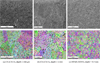 |
Fig. 3 Surface EBSD maps of the investigated steel measured after hardening treatment for CS and HFQS materials. Image Quality (IQ) maps (top) and Orientation maps using IPF notation for ND (bottom). Two distinct depths have been investigated for CS (a) and (b) and only one for HFQS (c). |
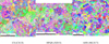 |
Fig. 4 EBSD orientation maps of the 3 investigated steels measured within the bulk of the samples after hardening. The boundaries corresponding to misorientations between 25° and 45° have been plotted as dark lines. |
3.3 Hardness measurements
The evolution of the hardness through the thickness is shown in Figure 5 before and after treatment for the CS and HFQS steels. In all cases, the plotted values have been averaged on 3 independent measurements, performed along 3 parallel lines from the surface through the material. The summary of the measured data at the extreme surface and within the bulk of the materials are given in Figure 6.
It is quite clear that all hardening treatments produce materials that are harder than the materials before processing (when documented) (an increase of hardness of 159 or 114 HV is observed for the CS and HFQS bulk materials), and that both treatments which aim at reinforcing the surface are also quite efficient (an additional increase of 222 and 301 HV is measured for CS and HFQS surface materials). The CS and HFQS are thus strongly reinforced on a thickness of few millimeters, whereas the AH treatment produces a constant and quite high hardness through the whole thickness of the material. If we assume an initial hardness around 250 HV similar to the one found in ferrite or bainite for the two other steels, then the AH treatment is associated with an additional hardness increase of about 300 HV. It is also seen in Figure 6 that the scatter of the measured values is larger on the surface than in the bulk of the materials. These values are in agreement with the literature for bainitic, ferritic and martensitic stainless steels (e.g. [35]).
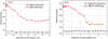 |
Fig. 5 Average (on 3 independent series) Vickers Hardness profiles before and after hardening treatment for the CS (left) and (b) HFQS (right) materials. |
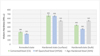 |
Fig. 6 Vickers Hardness (HV0.05) for all investigated samples, measured at the extreme surface and in the bulk of the materials. |
4 Quantitative analysis of the EBSD data
Now, in order to go further into the analysis of the microstructure, we need to extract some more quantitative data from the EBSD maps and specially to analyze in some details the grain size distribution as well as the misorientation profiles found after the 3 investigated thermal treatments, which are both directly linked to the transformation processes. Indeed, it is well-known that the transformation from an austenitic phase (which has a face-centered cubic structure (FCC) structure) to a martensitic or bainitic phase (which both present a body centered cubic (BCC) structure) usually obeys some crystallographic rules, which can be observed totally or only partially if some “variant selection” occurs during the process (see below). Different orientations relationships exist in the literature to describe the crystallographic orientation relationship (OR) between the parent phase (here the austenite) and the child phase (martensite). The most frequently cited are: the Bain OR [36], Kurdjimov-Sachs (KS) OR [37], Nishiyama-Wassermann (NW) OR [38,39] Greninger-Troiano (GT) OR [40] which is intermediate between KS and NW. Some other relationships are also reported in the literature, which are experimentally determined, like e.g. the CRB one [20,41], in bainite and which is also misoriented 3.4° and 4° from KS and NW, respectively. In fact, all these orientation relationships are quite close, since the KS, GT, CRB, Bain and NW relationships can be described by misorientations of 42.8, 44.2, 44.5, 45 and 46° respectively, around varying axes.
Additionally, each of the above-mentioned relationships is associated with a given number of possible so-called “variants”, which are the possible orientations of the child phase from one single parent orientation associated with one given relationship (whose maximum number is 24, because of the cubic symmetry). For the above-mentioned relationships, the number of possible variants is 24 for KS, GT and CRB, 12 for NW and 3 for Bain. A lot of experiments show that not all crystallographic variants are generated with equal frequency within a prior austenitic grain, and this is generally attributed to the so-called variant selection phenomenon [42]. This selection variant is generally observed both in bainite and martensite, with different selection rules though, and some authors propose a classification of the selected variants (and organization of the prior austenitic grains into blocks and packets) according to the composition of the steel, as well as the cooling rate [28]. In the case of the martensitic transformation, the displacive character of the transformation, i.e., occurring by a shear process instead of a diffusional one allows to attribute this variant selection to pre-existing stresses or strains. However, several mechanisms have already been proposed to explain this phenomenon of variant selection during the martensitic phase transformation. Pre-existing residual stresses within the austenite phase are frequently evoked to explain the selective nucleation of a limited number of variants during transformation [15,43]. Also, as the transformation itself from an FCC to a BCC crystal induces some local strains, the consideration of possible interactions between the residual stresses and these transformation strains is at the origin of several developing models of phase transformation [19,44]. But more simply, the observed variant selection can also be a result of an incomplete determination, especially when 2D microstructural observations are performed as it is usually the case using e.g. Scanning Electron Microscopy (SEM), whereas growth of variants is a 3D phenomenon [41].
In any case, this variant selection − which is rarely studied in stainless steels − can be highlighted by comparing the misorientation profile obtained within one (or few) prior austenitic grain(s) to the one obtained theoretically by considering, for one given orientation relationship, all possible misorientations between all variants, according to a widely used procedure [45]. This profile is presented in Figure 7 for the KS orientation relationship, which is the most widely accepted in (stainless) steels. This profile could correspond to the misorientation profile of GBs measured in one single prior austenitic grain, in which all variants are present in equal proportions. It is seen that for the KS orientation relationship, the major peak is expected around 50° (rarely found in martensite) and that no misorientation between variants is found between roughly 20° and 45° (strictly speaking, between 21.1 and 47.1, see Fig. 10). Consequently, the present inter-lath boundaries will be considered to be either Low Angle Grain Boundaries (LAGBs) for the misorientations below 20° or High Angle Grain Boundaries (HAGBs) for those above 45°. It is also worth recalling that the peak associated with 60° is partly associated with twin boundaries [28].
From the distribution of local misorientations (i.e., the misorientations calculated solely between neighbouring points), we have thus first extracted the percentage of the 3 possible classes of grain boundaries mentioned above, that is the LAGBs (associated with misorientations between 2° and 25°), the HAGBs (associated with misorientations between 45 and 62°) and the intermediate GBs (associated with misorientations between 20 and 45°). This has been done for two different individual maps for all examined states and the result is shown in Figure 8, whereas the averaged values are reported in Table 2. The error bar corresponds to the standard deviation calculated for each state on the two values obtained on the two examined maps. In this figure, some dashed and solid lines are also plotted which represent the expected percentages of these 3 GB categories for the KS relationship (30% for misorientations below 25°, 0% for misorientations between 25° and 45° and 70% for misorientations above 45°) as well as for a random orientation distribution (11% for misorientations below 25°, 47% for misorientations between 25° and 45° and 42% for misorientations above 45°).
It is first seen that the data extracted from 2 different maps for a same state may be quite scattered, since the standard deviation varies between 0.1 and 6 %. Some general trends are however visible;
None of these states are close to a random misorientation distribution even if the profiles associated with the surface maps appear closer to this random distribution.
These surface profiles are indeed quite different from the bulk ones, and contains more intermediate GBs than the bulk ones; this is expected from the examination of the complex microstructures in which grain growth during transformation is significantly perturbed by the presence of precipitates.
The highest HAGB % is obtained for 2 out of the 3 bulk martensitic microstructures (namely the ones obtained by cementation and high frequency quenching); the martensite obtained by age hardening presents a profile quite different and a HAGB percentage closer to the one found in bainite than in the other martensites (see Tab. 2).
As it was shown previously that the surface microstructures are more complex because of additional precipitation processes, the analysis will be continued only for the bulk microstructures and, in order to be more statistically relevant, the data presented are now averaged on all measured maps associated with the same state. These data are thus representative of zones of sizes varying between 20,000 and 80,000 μm2. For all bulk states, a representative grain size (GS) has first been extracted. In order to take into account all laths, the misorientation characterizing the distinction between grains and subgrains has been set equal to 10°, instead of the value of 15° classically considered. Given the fact that some different types of grain morphologies are seen in the investigated microstructures (either composed of more or less equiaxed grains or elongated laths), the choice has been made to characterize first the grain size by the average equivalent diameter (expressed in μm). Additionally, the average lath thickness − represented by the minimum diameter of the grains idealized by ellipses − has also been evaluated, especially for the martensitic states. Also, as seen in Table 2, as the standard deviation on the average grain size is quite large (of the same order as the GS itself), the weighted area average GS, i.e. weighted by the area of grains associated with a given value, is thought to be more significant in this case [46]. This representative grain size is quite different in the various microstructures. It is the largest for the bainite, and the smallest for one of the martensitic samples.
Additionally, it is seen in Figure 9a that there seems to be a unique correlation between the two selected size parameters for the 3 martensitic materials, which seems to be different for the ferrite and bainite states. Also, it is obvious from Figure 9b, that the presence of a high percentage of HAGBs in martensite reduces the grain size, just like the transformation from ferrite or bainite to martensite.
Some overall misorientation profiles have also been extracted from the large EBSD maps and are represented in Figure 10. By investigating the whole misorientation range from 2° to 62°, we necessarily include in these profiles the inter-laths misorientations when the microstructure is composed of lath packets, the classical GB misorientations for recrystallized microstructures (in ferrite for example), but also the inter-prior austenitic grains, when these are clearly visible in the maps. Additionally, the α/γ misorientations are also included when the material contains both phases.
A close inspection of this figure calls for the following comments:
The profiles found in bainite or ferrite indeed contain more “intermediate” GBs (i.e. between 25° and 45°) than those found in martensite; this could be due to the fact that the lath size is larger in these states than in martensite, resulting in turn to a larger influence of the prior austenitic GBs in the misorientation profiles; also the recrystallization in the ferrite has erased part of the orientation relationships due to the phase transformation.
The three martensitic profiles do present some major peaks around 55° or 60–62°. These peaks slightly differ from the theoretical ones calculated for the KS relationship (see Fig. 7). The agreement could be possibly better if we were considering a mixed KS and NW relationship, as in [47], although the justification of such a mixed approach appears still unclear.
The profile found in the MLX17 material appears significantly different from the other two martensitic profiles. Especially the percentage of HAGBs close to 60° is lower. This could be associated with the fact that this profile also contains a small percentage of α/γ boundaries, unlike the other two profiles, associated with 100% martensitic states.
These observations are consistent with Figure 8. These correlated profiles can also be compared with the theoretical one calculated by considering only the possible misorientations between variants due to KS relationship plotted in Figure 7. The comparison of both profiles is not trivial. However, by looking at Figure 7, we expect to see a major peak 50° if an equal proportion of variants is found within the whole map. Indeed, it is not the case in the investigated steels, and the major peak found for HAGBs is around 60° for the 3 martensitic states, which clearly indicates some variant selection during the martensitic transformation [24,48]. In order to explore this possibility, the analysis of the possible variants has been made according to the procedure developed by Takayama et al. [28] mainly for bainite. By considering the sole KS misorientation relationship, the 24 possible variants can be associated with 23 different inter-lath misorientations. These 23 misorientations can be further reduced to 16 distinct ones, since some variant couples do correspond to the very same misorientation (angle and axis). Then, the percentages of misorientations corresponding to these 16 misorientations can be extracted from the EBSD maps. This has been done for the 5 different bulk microstructures, i.e. the 3 martensitic states of interest, but also the 2 documented initial states, by again considering large maps (issued from the addition of several smaller maps) and a tolerance angle of 5°, and the results are presented in Figure 11 (for bainite and ferrite) and Figure 12 (for martensite). The obtained percentages have also been added to Table 2. They could appear quite small, but this is due to the fact that they represent the percentages of the 23 possible misorientations out of all misorientations calculated for all couples of neighbouring points within an EBSD map (including thus a lot of very small misorientations associated with the couples of points located within the same grain or lath), and not by considering the sole grain boundaries.
Figures 11 and 12 contain thus the percentage of the 23 possible misorientations between variant 1 and variants 2 to 24, whose order is strictly the same as the one proposed by Takayama et al. [28]. The variants are thus classically grouped so that they are associated with the same {111} plane in the austenitic phase 6 by 6. Also, the 7 variants associated with variant 1 in the same Bain zone and associated with misorientations less than 25° are identified in the figures. In other words, variants 1 to 6 are associated with the same {111}α plane whereas variants 1, 4, 8, 11, 13, 16, 21 and 24 are within the same Bain zone. Misorientation V1/V2 corresponds to a misorientation of 60° around a {111}α plane (twin boundary), whereas V1/V3 or V1/V5 correspond to 60° rotation around a {110}α plane. In both figures, the four main peaks associated with high or low misorientations are identified by arrows (in black for the HAGBs corresponding to 60° misorientation and red for the LAGBs corresponding to variants belonging to the same Bain zone). It is interesting to note that in all microstructures, the 4 main peaks are the same; in other words, the principal misorientations associated with KS variants are the same in ferrite, bainite or martensite. This observation could be directly linked to the actual composition of the materials [49], and especially to the actual C content. However, the previously published data are somewhat contradictory. Indeed, a high percentage of V1/V2 misorientations have been found either for a high C content (around 1.8%) [49] or a low C content (equal to 0.17%) [47]. In any case, we can already conclude that, in all cases, we do observe a transformation process close to KS relationship and some variant selection, as expected from a displacive transformation. The observed variant selection is different though from the one usually observed in martensite for low C steels − for which the main variant pairs are generally associated with low misorientations − but has occasionally been observed in some other stainless steels [11,47]. We can thus conclude at this point that this variant selection cannot be simply related to the C content.
Of course, the exact percentage of the observed inter-variant misorientations depends on the retained orientation relationship as well as on the calculation procedure (and especially the tolerance angle, see e.g. [49]). But in the present case, whatever the procedure, the variant V1/V2 is always more present than the other variants, in agreement with the misorientation profiles presented in Figure 10. Usually, this variant pair is more frequently reported for bainite transformed at high temperature [28], whereas variants pairs such as V1/V4 or V1/V8 and associated with small misorientations and the same Bain group are much more often reported for martensite [45,49–51]. These observations are often tentatively explained by the so-called Phenomenological Transformation Martensite Crystallography theory [16,17,45] which allows to calculate the transformation strain associated with one single variant or a combination of 2 or more variants. Depending on the actual value of the resulting strain (see Tab. 3), the variant combination is said to accommodate the transformation more or less efficiently. Especially, if all 6 variants associated with the same plane are present, the overall strain is very small [52]. The accommodation is also better for V1/V4 pair than for the V1/V2 pair, which does correspond to a quite large strain, compared to any other couple (see Tab. 3). It is hard in the present case to validate the presence of one variant pair or another by this simple theory which considers an isolated variant pair, since the actual texture of the parent phase and the neighbouring grains of each austenite prior grain should be taken into account in order to predict the overall strain due to the transformation. Some other studies, also based on the selection of specific variants, try to explain the observed ones by the minimization of the elastic energy [53]. In the present case, as the transformation conditions are poorly documented, it seems inappropriate to attempt to justify the presence of this variant pair V1/V2 by such simple theories, but we think that the presence of this variant, associated with a lot of TBs, affects the mechanical response of the stainless steels.
Indeed, these TBs are quite special boundaries. Although there are associated with a high angle misorientation, and thus thought to be quite resistant to dislocation movements across these boundaries, due to the associated specific misorientation (60° around a {111}α direction), the two orientations sharing such a TB do have a lot of slip traces in common. This can have the opposite effect of facilitating the passage of dislocations from one grain to another, and thus of reducing in turn the hardening effect of grain size reduction (so-called Hall Petch effect). This is illustrated in Figure 13, in which all possible slip plane normals (called poles in a stereographic projection) have been plotted for two couples of orientations V1/V2 and V1 /V4, by considering the cube orientation for V1 (i.e., the orientation for which the {100} directions coincide with the 3 directions constituting the sample reference frame, RD, TD and ND). For each orientation, we have thus 6 {110} poles and 12 {112} poles, which have been plotted separately for sake of clarity. The poles associated with the cube orientation are represented by crosses, whereas those associated with the other two orientations misoriented according to V2 (60°<111>) or V4 (10.5°<110>) are represented by black dots. It is clearly seen that the V1 and V2 variants possess six slip plane normals in common (3 {110} and 3 {112}) whereas the V1 and V4 variants possess only one {110} slip plane normal in common. All other normals are slightly misoriented (10.5°). During plastic strain, these two different configurations will have a different effect on both yield strength and hardening evolution, depending on the loading path: for some loading conditions, the HAGBs associated with V1/V2 may appear to be softer than the LAGBs associated with V1/V4.
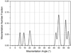 |
Fig. 7 Normalized misorientation profile calculated for all possible variants associated with the KS misorientation relationship (24 variants associated with 23 misorientations associated with 10 different misorientation angles [28]). |
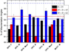 |
Fig. 8 Percentages of low, intermediate and high misorientations found in the various investigated maps. The error bar corresponds to the standard deviation. The dashed lines correspond to the values associated with only KS misorientations and the solid lines correspond to the values found in a random orientation distribution. |
Microstructural parameters extracted from the EBSD maps.
 |
Fig. 9 Correlation between (a) average GS and lath thickness and (b) HAGB percentage and average GS. Associated with the designation of the steel, F stands for ferrite, B for bainite and M for martensite. |
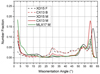 |
Fig. 10 Normalized correlated misorientation profiles before and after hardening process for the 3 martensitic steels. F stands for ferrite, B for bainite and M for martensite. |
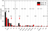 |
Fig. 11 Calculated percentages of KS inter-variant misorientations for the two initial states (CX13 and XD15 materials) before martensitic transformation. |
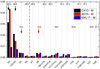 |
Fig. 12 Calculated percentages of KS inter-variant misorientations for the three martensitic states (CX13, XD15 and MLX17 materials). |
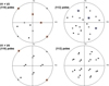 |
Fig. 13 Slip plane {110} and {112} normals plotted in stereographic projection for couples of orientations associated with variants V1+V2 or V1+V4. The small crosses correspond to variant V1 (Cube orientation), and the black dots to variants V2 or V4. The red circles highlight the common {110} poles whereas the blue ones highlight the common {112} poles. |
5 Correlation between microstructure and yield strength
It may thus be of interest to try to establish a link between the collected microstructural data and the final hardness of the martensite, which has been observed to be quite high, both in surface and within the bulk of the materials, compared to the initial bainite or ferrite. We can say that the main hardening mechanisms in such steels can be (i) the reduction of the grain size during martensitic transformation (σGS due to the Hall-Petch effect), (ii) the presence of dislocations due to the displacive transformation (σρ), and the effect of alloying elements in the form of (iii) a solid solution (σSS)or (iv) precipitates (σPrec). We can first estimate the yield stress (σYS) from the micro-hardness, from the following relationship identified by Pavlina and Vantyne [54]
 (1)
(1)
The calculated values are reported in Table 4 where it is seen that all microstructural states are associated with quite high σYS values: the reference value (when available) is estimated between 600 and 730 MPa, the bulk thermal treatment leads to an increase of 400 to 600 MPa and the surface treatment induces an additional increase of the order of 600 to 800 MPa. We can thus say, before going further, that the contribution of the surface treatment is already larger that the sole effect of the bulk thermal treatment for both CX13 and XD15 steels. Based on the above detailed microstructural observations, we can also assume that the principal sources of hardening are somewhat different for the various investigated microstructures (see Tab. 4).
If we compare specifically the three bulk martensite states, it is seen that if the sole martensitic transformation may have an influence on hardening, the additional presence of alloying elements (and especially the C) may affect differently the hardening, depending on the way these are present in the material. For example, we expect a major hardening contribution from the presence of (nano)-precipitates in MLX17, whereas the contribution will come mainly from the alloying elements in solid solution in CX13, in which no precipitate could be identified within the bulk martensitic material. The situation is less clear for the XD15 material, in which the C percentage is quite high, and a limited number of precipitates has been observed after hardening treatment.
Classically, to account for such hardening contributions, an additive expression is often adopted for the yield stress, such as, according to [9–11,27,55]
 (2)
(2)
Unfortunately, there is not one unique way of evaluating each of the listed contributions, which are far from being strictly independent from each other. Especially, the exact contribution of the alloying elements in solid solution (σSS) or as precipitates (σPrec) would require “burdensome measurements” as mentioned by Zeng et al. [11], which moreover were inaccessible to us. The adopted procedure consists thus, as in references [9–11,27,55], to evaluate all contributions that can be evaluated separately with satisfactory precision and to deduce the remaining ones from the macroscopic measurement of σYS. In what follows, we are going to evaluate the first two terms in equation (2) in an approximate way for the 3 bulk martensites only, since the same evaluation for the surface materials would necessitate a more detailed chemical analysis after cementation or HF quenching.
Let us consider first the influence of the grain size on the yield stress; this usually obeys the so-called Hall-Petch relation, classically written as
 (3)
(3)
If it were the sole hardening mechanism, this relation would imply that the yield stress varies linearly with the inverse square root of the mean grain size. Indeed, one such single correlation is not seen in the present study, when we consider all investigated states (see Fig. 14). For the sole martensitic states, we do observe instead a decrease of σYS with the decrease of the grain size (whatever the representative GS); in other words, we cannot isolate the sole contribution of the grain size from the evaluation of the yield stress. This obvious fact has already been noticed by other authors [56], and could be due partly to the contradictory effects of the massive presence of twin boundaries.
To describe the GS effect on yield strength, we thus adopt the Hall–Petch relation proposed by Hutchinson et al. [27] with σ0 = 150 MPa and k = 189 when the grain size is expressed in μm. These coefficients has been assessed on dislocated ferrite, which is thought to be well adapted to the estimation of a “reference” Hall − Petch law for martensite and which is consistent with other values found in the literature for somewhat similar materials [9,11,56,57]. The GS effect has then been calculated for both representative quantities, that is the lath size or the weighted average grain size. The first parameter is more widely accepted in the literature when considering martensitic steels (i.e., [56,57]).
Then, the hardening due to a given dislocation density ρ is classically described by
 (4)
(4)
where G = 80 GPa is the shear modulus, b = 0.25 nm is the magnitude of the Burgers vector and α is a constant having the value of about 0.24 [58]. The dislocation density has been evaluated according to two different procedures. First, following Hutchinson et al. [27], we estimate it from the linear dependance observed by Morito et al. [59] between dislocation density and C content in solid solution.
 (5)
(5)
A second estimation of dislocation density can be made from the EBSD maps, but it then concerns solely the geometrically necessary dislocations (GND), i.e. the ones associated with misorientations at grain or subgrain boundaries [60]. The local density of GND is classically described by the following expression
 (6)
(6)
in which θ is the misorientation at the considered point, Δ the distance between two measurements, b the magnitude of the Burgers vector and β a constant that depends on the type of dislocations. It has been shown in a recent study [61] that this parameter should be taken equal to 3 for cubic metals. The misorientation is then most often represented by the KAM (Kernel Average Misorientation) parameter by considering 1 to 3 EBSD measurement steps for Δ (we have considered 3 steps in the present case, in order to obtain a satisfactory precision). This parameter is an estimate of the local misorientation, calculated as the average of the misorientations between one given point and its nearest neighbors, excluding those which are not located within the same grain.
The GS and ρ contributions arising directly from the martensitic transformation are listed in Table 5. For the evaluation of the C percentage in SS for the XD15 steel which contains some carbides, we have taken an approximate value (the same as in the CX13 steel which does not contain any precipitate). It is interesting to note that both evaluations of σρ are of the same order of magnitude and quite small indeed (but fully consistent with the quality of the EBSP maps). For the GS contribution, the trend is also the same for both selected parameters, but the contribution is larger when considering the lath thickness. If we consider that this last parameter is more appropriate for martensite, and by taking the dislocation density estimated from the KAM, which contains less uncertainty than the one estimated from the C content, we end up with a remaining contribution σrem due mainly to the effect of the alloying elements in the form of solid solution or precipitates and calculated as:
 (7)
(7)
As the percentage of precipitates is quite small in the XD15 material (1.1%) and has thus a negligible influence on hardening (indeed, by considering the approach developed by Ohlund et al. for precipitates [55], we find a contribution of 7 MPa), we can conclude that this remaining hardening contribution is mainly due to the C remaining in solid solution for both CX13 and XD15 steels, whereas it is mainly due to the presence of nanoprecipitates for the MLX17 material. The exact percentage of C remaining in solid solution is not known though for the XD15 material, which contains a small proportion of carbides.
We can now compare these remaining contributions obtained in the present case to the ones found by Hutchinson et al. [27] for the same C percentages. This can be done easily for the CX13 material, which does not contain any precipitate, and which thus contains 0.15% C in solid solution. For this case, we find however a smaller contribution than the one estimated in reference [27] (534 MPa for the present study versus 760 MPa). These authors argue that the hardening effect is due to the segregation of the carbon atoms to dislocations and lath boundaries which affects the movement of mobile dislocations as though they were in true solid solution, or even more. In the present case, the segregation at TBs (whose percentage is quite high in both steels) could be less than at general HAGBs, thus reducing the hardening influence of the segregated atoms, in the present case. Similarly, we can also compare the hardening effect of solid solution for the two materials for which it is thought to be the sole contribution of the alloying elements, that is the CX13 and XD15 materials. The small remaining hardening contribution for the XD15 material (233 MPa compared to 888 MPa for the MLX17 material) is indeed a bit surprising. But again, the presence of more twin boundaries in this material than in the CX13 alloy (4.4% versus 3.1%) could have led to an overestimation of the GS effect and an underestimation in turn of the SS influence. This means that equations (2) or (3) should be modified to take into account not only the grain size but also the influence of specific boundaries. This will imply an additional study on more than only 3 different microstructural states.
Estimated yield strength and principal sources of hardening for the various microstructures.
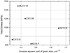 |
Fig. 14 Hall–Petch plot relating yield stress to inverse square root of the grain size in terms of the average weighted area grain size (in μm). |
Estimated hardening contributions in martensite.
6 Conclusions
The present study has detailed the martensitic structures found in 3 different stainless steels, developed for their mechanical, corrosion and wear resistances. A link between the microstructural features and the resulting yield stress is then proposed. The main conclusions of this study are:
For the 3 investigated materials, the martensitic transformation obeys the classical KS orientation relationship, but some variant selection is observed and the microstructures look different in terms of grain size and orientation distributions.
This variant selection produces a relatively high proportion of twin boundaries, especially in the 2 steels containing the highest C percentage (CX13 and XD15).
This specific variant selection, which has occasionally been observed in some other stainless steels, is different from the one usually reported in the low C steels. It is generally attributed to the variation on the martensitic transformation temperature with C content.
Apart from the grain size and dislocation contributions, the main remaining hardening contribution is due to the segregation of C atoms at lath boundaries for the CX13 and XD15 steels, whereas it is due to the presence of nanoprecipitates for the MX17 material.
The link between these microstructural features, hardening mechanisms and tribological properties will be detailed in a forthcoming paper.
Declaration of competing interest
The authors declare that they have no known competing financial interests or personal relationships that could have appeared to influence the work reported in this paper.
Data availability
The raw/processed data required to reproduce these findings cannot be shared at this time as the data also forms part of an ongoing research project.
Acknowledgements
The authors would like to thank BPI and Conseil Général 93 for the financial support of this research, in the framework of the FUI11 project MEKINOX. They also acknowledge the contribution of all industrial and academic partners of the MEKINOX project to the elaboration of the studied samples, and to fruitful discussions around the work detailed in the present manuscript.
References
- E. Soujanya, B.N. Sarada, Effects of age hardening on the mechanical properties of high silicon stainless steel, Mater. Today Proc. 46, 4362–4367 (2021) [CrossRef] [Google Scholar]
- L. Bao, J. Chen, Q. Li et al., Research on a new localized induction heating process for hot stamping steel blanks, Materials 12, 1024 (2019) [CrossRef] [PubMed] [Google Scholar]
- D. Ghiglione, C. Leroux, C. Tournier, Cémentation. Carbonitruration. Techniques de l’ingénieur M1226, pp. 1–45 (1994) [Google Scholar]
- Y. Liu, M. Wang, J. Shi et al., Fatigue properties of two case hardening steels after carburization, Int. J. Fatigue 31, 292–299 (2009) [CrossRef] [Google Scholar]
- H.J. Lee, H. Kil, S.H. Kim et al., Corrosion and carburization behavior of chromia-forming heat resistant alloys in a high-temperature supercritical-carbon dioxide environment, Corros. Sci. 99, 227–239 (2015) [CrossRef] [Google Scholar]
- Y.-H. Yang, M. Wang, J.-C. Chen et al., Microstructure and mechanical properties of gear steels after high temperature carburization, J. Iron Steel Res. Int. 20, 140–145 (2013) [CrossRef] [Google Scholar]
- H.J. Kang, J.S. Yoo, J.T. Park et al., Effect of nano-carbide formation on hydrogen-delayed fracture for quenching and tempering steels during high-frequency induction heat treatment, Mater. Sci. Eng. A 543, 6–11 (2012) [CrossRef] [Google Scholar]
- S. Kikuchi, A. Sasago, J. Komotori, Effect of simultaneous surface modification process on wear resistance of martensitic stainless steel, J. Mater. Process. Technol. 209, 6156–6160 (2009) [CrossRef] [Google Scholar]
- H. Luo, X. Wang, Z. Liu et al., Influence of refined hierarchical martensitic microstructures on yield strength and impact toughness of ultra-high strength stainless steel, J. Mater. Sci. Technol. 51, 130–136 (2020) [CrossRef] [Google Scholar]
- C. Wang, K. Luo, J. Wang et al., Carbide-facilitated nanocrystallization of martensitic laths and carbide deformation in AISI 420 stainless steel during laser shock peening, Int. J. Plast. 150, 103191 (2022) [CrossRef] [Google Scholar]
- T.Y. Zeng, W. Li, N.M. Wang et al., Microstructural evolution during tempering and intrinsic strengthening mechanisms in a low carbon martensitic stainless bearing steel, Mater. Sci. Eng. A 836, 142736 (2022) [CrossRef] [Google Scholar]
- K.H. Lo, C.H. Shek, J.K.L. Lai, Recent developments in stainless steels, Mater. Sci. Eng. R 65, 39–104 (2009) [CrossRef] [Google Scholar]
- G. Kalwa, E. Schnabel, P. Schwaab, Grain structure of bainitic and martensitic steels, Steel Res. 57, 207–215 (1986) [CrossRef] [Google Scholar]
- R. Badji, B. Bacroix, M. Bouabdallah, Texture, microstructure and anisotropic properties in annealed 2205 duplex stainless steel welds, Mater. Charact. 62, 833–843 (2011) [CrossRef] [Google Scholar]
- G. Miyamoto, N. Iwata, T. Takayama et al., Quantitative analysis of variant selection in ausformed lath martensite, Acta Mater. 60, 1139–1148 (2012) [CrossRef] [Google Scholar]
- S. Morito, H. Tanaka, R. Konichi et al., The morphology and crystallography of lath martensite in Fe-C alloys, Acta Mater. 51, 1789–1799 (2003) [CrossRef] [Google Scholar]
- S. Morito, H. Yoshida, T. Maki et al., Effect of block size on the strength of lath martensite in low carbon steels, Mater. Sci. Eng. A 438–440, 237–240 (2006) [CrossRef] [Google Scholar]
- O. Haiko, V. Javaheri, K. Valtonen et al., Effect of prior austenite grain size on the abrasive wear resistance of ultra-high strength martensitic steels, Wear 203336 (2020) [CrossRef] [Google Scholar]
- L. Qi, A.G. Khachaturyan, J.W. Morris Jr, The microstructure of dislocated martensitic steel: theory, Acta Mater. 76, 23–39 (2014) [CrossRef] [Google Scholar]
- C. Cabus, H. Réglé, B. Bacroix, Orientation relationship between austenite and bainite in a multiphased steel, Mater. Character. 58, 332–338 (2007) [CrossRef] [Google Scholar]
- R.K. Ray, M.P. Butron-Guillén, J.J. Jonas, Transformation textures in a controlled rolled Nb-V steel, Texture Microstruct. 14–18, 483–491 (1991) [CrossRef] [Google Scholar]
- K. Zhu, O. Bouaziz, C. Oberbillig et al., An approach to define the effective lath size controlling yield strength of bainite, Mater. Sci. Eng. A 527, 6614–6619 (2010) [CrossRef] [Google Scholar]
- Z. Guo, C.S. Lee, J.W. Morris Jr, On coherent transformations in steel, Acta Mater. 52, 5511–5518 (2004) [CrossRef] [Google Scholar]
- S. Morito, H. Tanaka, R. Konishi et al., The morphology and crystallography of lath martensite in alloy steels, Acta Mater. 54, 5323–5331 (2006) [CrossRef] [Google Scholar]
- J.W.J. Morris Jr, C. Kinney, K. Pytlewski et al., Microstructure and cleavage in lath martensitic steels, Sci. Technol. Adv. Mater. 14, 014208 (2013) [CrossRef] [PubMed] [Google Scholar]
- K. Zhu, D. Barbier, T. Iung, Characterization and quantification methods of complex BCC matrix microstructures in advanced high strength steels, J. Mater. Sci. 48, 413–423 (2013) [CrossRef] [Google Scholar]
- B. Hutchinson, J. Hagström, O. Karlsson et al., Microstructures and hardness of as-quenched martensites (0.1–0. 5%C), Acta Mater. 59, 5845–5858 (2011) [CrossRef] [Google Scholar]
- N. Takayama, G. Miyamoto, T. Furuhara, Effects of transformation temperature on variant pairing of bainitic ferrite in low carbon steel, Acta Mater. 60, 2387–2396 (2012) [CrossRef] [Google Scholar]
- A. Martinavicius et al., Caractérisations microstructurales des aciers MEKINOX par sonde atomique et MEB, I. Report, Editor 2013, Normandie Univ., UNIROUEN, INSA Rouen, CNRS, Groupe de Physique des Matériaux, Rouen 76000, France [Google Scholar]
- A. Bénéteau, Étude in situ des évolutions microstructurales d’un acier inoxydable martensitique à l’azote au cours d’une succession de traitements thermiques, Institut National Polytechnique de Lorraine, 2007 [Google Scholar]
- T. Santos, Contribution à la compréhension des liens entre microstructure et propriétés tribologiques d’aciers inoxydables haute dureté après traitements de surface, University Paris13, 2015 [Google Scholar]
- G. Ebrahimi, A. Momeni, M. Jahazi et al., Dynamic recrystallization and precipitation in 13Cr super-martensitic stainless steels, Metall. Trans. A 45, 2219–2231 (2014) [CrossRef] [Google Scholar]
- N. Fujita, K. Ohmura, A. Yamamoto, Changes of microstructures and high temperature properties during high temperature service of Niobium added ferritic stainless steels, Mater. Sci. Eng. A 351, 272–281 (2003) [CrossRef] [Google Scholar]
- D. Pye, Practical Nitriding and Ferritic Nitrocarburizing, ASM International, Materials Park, OH, 2003, p. 159 [Google Scholar]
- V.I. Belyakova, M.F. Alekseenko, Structure and properties of carburized martensite stainless steels, Metal Sci. Heat Treat. 11, 32–34 (1969) [CrossRef] [Google Scholar]
- E.C. Bain, The nature of martensite, Trans. AIME Steel Divis. 70, 25–46 (1924) [Google Scholar]
- G. Kurdjumov, G. Sachs, Über den Mechanismus der Stahlhärtung, Zeitsch. Phys. 64, 325–343 (1930) [CrossRef] [Google Scholar]
- G. Wasserman, Uber den Mechanismus der α-γ-Umwandlung des Eisens, Arch. Eisenhüttenwes 16, 647 (1933) [Google Scholar]
- Z. Nishiyama, X-ray investigation o the mechanism of the transformation from face-centred cubic lattice to body-centered cubic, in Scientifc Report Tohoku Imperial University, 1935 p. 637 [Google Scholar]
- A.B. Greninger, A.R. Troiano, The mechanism of martensite formation, Metals Trans. 185, 5–15 (1949) [Google Scholar]
- C. Cabus, H. Réglé, B. Bacroix, The influence of grain morphology on texture measured after phase transformation in multiphase steels, J. Mater. Sci. 49, 5646–5657 (2014) [CrossRef] [Google Scholar]
- H. Inagaki, in Proc. 6th inst. Conf. on Textures of Materials (1981) p. 149 [Google Scholar]
- M. Ueda, H. Yasuda, Y. Umakoshi, Effect of grain boundary on martensite transformation behaviour in Fe-32 at.%Ni bicrystals, Sci. Technol. Adv. Mater. 3, 171–179 (2002) [CrossRef] [Google Scholar]
- P. Bate, B. Hutchinson, The effect of elastic interactions between displacive transformations on textures in steels, Acta Mater. 48, 3183–3192 (2000) [CrossRef] [Google Scholar]
- A. Lambert-Perlade, A.F. Gourgues, A. Pineau, Austenite to bainite phase transformation in the heat-affected zone of a high strength low alloy steel, Acta Mater. 52, 2337–2348 (2004) [CrossRef] [Google Scholar]
- B. Bacroix, S. Queyreau, D. Chaubet et al., The influence of the cube component on the mechanical behaviour of copper polycrystalline samples in tension, Acta Mater. 160, 121–136 (2018) [CrossRef] [Google Scholar]
- B. Sonderegger, S. Mitsche, H. Cerjak, Martensite laths in creep resistant martensitic 9-12% Cr steels — calculation and measurement of misorientations, Mater. Character. 58, 874–882 (2007) [CrossRef] [Google Scholar]
- P.P. Suikkanen, C. Cayron, A.J. DeArdo et al., Crystallographic analysis of isothermally transformed bainite in 0.2C-2.0Mn-1.5Si-0.6Cr steel using EBSD, J. Mater. Sci. Technol. 29, 359–366 (2013) [CrossRef] [Google Scholar]
- A. Stormvinter, G. Miyamoto, T. Furuhara et al., Effect of carbon content on variant pairing of martensite in Fe―C alloys, Acta Mater. 60, 7265–7274 (2012) [CrossRef] [Google Scholar]
- S. Morito, A.H. Pham, T. Hayashi et al., Block boundary analyses to identify martensite and bainite, Mater. Today Proc. 2, S913–S916 (2018) [Google Scholar]
- C.C. Kinney, K.R. Pytlewski, A.G. Khachaturyan et al., The microstructure of lath martensite in quenched 9Ni steel, Acta Mater. 69, 372–385 (2014) [CrossRef] [Google Scholar]
- V. Pancholi, M. Krishnan, I. Samajdar et al., Self-accommodation in the bainitic microstructure of ultra-high-strength steel, Acta Mater. 56, 2037–2050 (2008) [CrossRef] [Google Scholar]
- F. Maresca, W.A. Curtin, The austenite/lath martensite interface in steels: structure, athermal motion, and in-situ transformation strain revealed by simulation and theory, Acta Mater. 134, 302–323 (2017) [CrossRef] [Google Scholar]
- E.J. Pavlina, C. Vantyne, Correlation of yield strength and tensile strength with hardness for steels, J. Mater. Eng. Perform. 17, 888–893 (2008) [CrossRef] [Google Scholar]
- C.E.I.C. Ohlund, D. den Ouden, J. Weidow et al., Modelling the evolution of multiple hardening mechanisms during tempering of Fe-C-Mn-Ti martensite, Isij Int. 55, 884–893 (2015) [CrossRef] [Google Scholar]
- C. Sun, P. Fu, H. Liu et al., The effect of lath martensite microstructures on the strength of medium-carbon low-alloy steel, Crystals 10, 232 (2020) [Google Scholar]
- J. Hidalgo, M.J. Santofimia, Effect of prior austenite grain size refinement by thermal cycling on the microstructural features of As-quenched lath martensite, Metall. Mater. Trans. A 47, 5288–5301 (2016) [CrossRef] [Google Scholar]
- N. Hansen, X. Huang, Microstructure and flow stress of polycrystals and single crystals, Acta Mater. 46, 1827–1836 (1998) [CrossRef] [Google Scholar]
- S. Morito, J. Nishikawa, T. Maki, Dislocation density within lath martensite in Fe-C and Fe-Ni alloys, Isij Int. 43, 1475–1477 (2003) [CrossRef] [Google Scholar]
- J. Jiang, T.B. Britton, A.J. Wilkinson, Evolution of dislocation density distributions in copper during tensile deformation, Acta Mater. 61, 7227–7239 (2013) [CrossRef] [Google Scholar]
- P.J. Konijnenberg, S. Zaefferer, D. Raabe, Assessment of geometrically necessary dislocation levels derived by 3D EBSD, Acta Mater. 99, 402–414 (2015) [CrossRef] [Google Scholar]
Cite this article as: Thiago Santos, Danièle Chaubet, Tony Da Silva Botelho, Guillaume Poize, Brigitte Bacroix, Analysis of the microstructural features of phase transformation during hardening processes of 3 martensitic stainless steels, Metall. Res. Technol. 120, 117 (2023)
All Tables
Estimated yield strength and principal sources of hardening for the various microstructures.
All Figures
|
Fig. 1 EBSD orientation maps of the CS (a) and HFQS (b) materials determined before hardening treatment. The microstructure is bainitic for the CS steel (a) and ferritic for the HFQS steel (b). The color corresponds to the crystallographic orientation of the ND direction within the crystal reference frame, according to the color code given by the unit triangle. For both microstructures, the step size is equal to 0.2 μm and the boundaries corresponding to misorientations between 25° and 45° have been plotted as dark lines. |
| In the text | |
|
Fig. 2 Image Quality (IQ) Index maps of the CS (a) and HFQS (b) materials determined before hardening treatment. |
| In the text | |
|
Fig. 3 Surface EBSD maps of the investigated steel measured after hardening treatment for CS and HFQS materials. Image Quality (IQ) maps (top) and Orientation maps using IPF notation for ND (bottom). Two distinct depths have been investigated for CS (a) and (b) and only one for HFQS (c). |
| In the text | |
|
Fig. 4 EBSD orientation maps of the 3 investigated steels measured within the bulk of the samples after hardening. The boundaries corresponding to misorientations between 25° and 45° have been plotted as dark lines. |
| In the text | |
|
Fig. 5 Average (on 3 independent series) Vickers Hardness profiles before and after hardening treatment for the CS (left) and (b) HFQS (right) materials. |
| In the text | |
|
Fig. 6 Vickers Hardness (HV0.05) for all investigated samples, measured at the extreme surface and in the bulk of the materials. |
| In the text | |
|
Fig. 7 Normalized misorientation profile calculated for all possible variants associated with the KS misorientation relationship (24 variants associated with 23 misorientations associated with 10 different misorientation angles [28]). |
| In the text | |
|
Fig. 8 Percentages of low, intermediate and high misorientations found in the various investigated maps. The error bar corresponds to the standard deviation. The dashed lines correspond to the values associated with only KS misorientations and the solid lines correspond to the values found in a random orientation distribution. |
| In the text | |
|
Fig. 9 Correlation between (a) average GS and lath thickness and (b) HAGB percentage and average GS. Associated with the designation of the steel, F stands for ferrite, B for bainite and M for martensite. |
| In the text | |
|
Fig. 10 Normalized correlated misorientation profiles before and after hardening process for the 3 martensitic steels. F stands for ferrite, B for bainite and M for martensite. |
| In the text | |
|
Fig. 11 Calculated percentages of KS inter-variant misorientations for the two initial states (CX13 and XD15 materials) before martensitic transformation. |
| In the text | |
|
Fig. 12 Calculated percentages of KS inter-variant misorientations for the three martensitic states (CX13, XD15 and MLX17 materials). |
| In the text | |
|
Fig. 13 Slip plane {110} and {112} normals plotted in stereographic projection for couples of orientations associated with variants V1+V2 or V1+V4. The small crosses correspond to variant V1 (Cube orientation), and the black dots to variants V2 or V4. The red circles highlight the common {110} poles whereas the blue ones highlight the common {112} poles. |
| In the text | |
|
Fig. 14 Hall–Petch plot relating yield stress to inverse square root of the grain size in terms of the average weighted area grain size (in μm). |
| In the text | |
Current usage metrics show cumulative count of Article Views (full-text article views including HTML views, PDF and ePub downloads, according to the available data) and Abstracts Views on Vision4Press platform.
Data correspond to usage on the plateform after 2015. The current usage metrics is available 48-96 hours after online publication and is updated daily on week days.
Initial download of the metrics may take a while.